
If you have ever built a survey, a questionnaire, or a psychological test, you have probably asked yourself one question: can I trust these scores? That is the core question behind split-half reliability, one of the oldest and most intuitive methods for checking whether a measurement instrument is internally consistent.
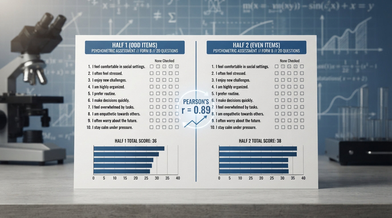
Split-half reliability divides a test into two halves, scores each half separately, and then correlates the two sets of scores. A high correlation tells you the items are measuring the same underlying construct. A low correlation is a warning sign that your test may be unstable or poorly constructed.
Despite the rise of Cronbach’s alpha as the default reliability statistic in most statistical software, split-half reliability has not disappeared. It remains useful in specific scenarios where alpha falls short, and it provides a transparency that more complex formulas sometimes obscure. In this guide, our team breaks down exactly how split-half reliability works, walks through a worked numerical example, and explains when you should still reach for it in 2026.
Table of Contents
Quick Answer: What Is Split-Half Reliability?
Split-half reliability is a measure of internal consistency that works by dividing a test into two halves, computing scores for each half, and correlating them using the Pearson correlation coefficient. The correlation is then adjusted upward using the Spearman-Brown prophecy formula to estimate the reliability of the full-length test rather than just half of it.
It falls under the family of internal consistency reliability methods within classical test theory. Unlike test-retest reliability, which requires administering the same test twice to the same group, split-half reliability needs only a single test administration. That makes it faster and cheaper to compute, which is one reason it remains popular in survey validation, questionnaire reliability studies, and educational assessment contexts.
The method was first formalized in the early 20th century alongside the broader development of psychometric analysis. Charles Spearman introduced the correction formula that bears his name in 1910, and the split-half technique itself grew out of efforts to understand whether test items were functioning as parallel measures of a single construct. More than a century later, researchers, graduate students, and test developers still rely on it for quick, interpretable checks on scale consistency.
How Split-Half Reliability Works: The 3-Step Process
The split-half method is refreshingly simple compared to many psychometric procedures. You can compute it by hand if needed, which is part of its enduring appeal. Here is how split-half reliability works in three steps.
Step 1: Split the Test into Two Halves
Take your full set of test items and divide them into two comparable halves. The goal is to create two mini-tests that are as similar as possible in content, difficulty, and number of items. If your test has 20 items, each half should contain 10 items covering the same construct.
There are three common ways to do this split, which we cover in detail in the next section. The odd-even split is the most widely used because it naturally balances content across the entire test.
Step 2: Score Each Half Separately
For every respondent in your sample, calculate a total score for the first half and a total score for the second half. If you have 50 respondents, you will end up with two columns of 50 scores each. One column represents performance on the odd-numbered items, and the other represents performance on the even-numbered items (or whatever split method you chose).
This step is straightforward in any spreadsheet or statistical package. In Excel, you would simply sum the relevant columns for each respondent.
Step 3: Correlate the Two Halves and Apply Spearman-Brown
Compute the Pearson correlation coefficient between the two sets of half-test scores. This correlation tells you how consistently the two halves rank-order your respondents. A correlation of 0.80 means the two halves are largely in agreement about who scored high and who scored low.
But there is a catch. Each half is only half the length of the original test, and shorter tests are inherently less reliable. So the raw correlation systematically underestimates the reliability of the full test. The Spearman-Brown prophecy formula corrects this by estimating what the reliability would be if the test were at its full length.
The adjusted reliability coefficient is your final split-half reliability estimate for the full instrument.
Methods of Splitting a Test
The way you split your test matters more than most people realize. Different splitting methods can produce noticeably different reliability estimates because they group items differently. Here are the three main approaches.
Odd-Even Split
The odd-even split assigns odd-numbered items (1, 3, 5, 7…) to one half and even-numbered items (2, 4, 6, 8…) to the other. This is the most popular method because it naturally distributes content evenly across both halves. If test difficulty or item quality changes gradually from the beginning to the end of the test, the odd-even split ensures both halves capture that full range.
First-Half / Last-Half Split
The first-half last-half split puts items 1 through N/2 in one group and items N/2+1 through N in the other. This method is simple but problematic if fatigue effects, practice effects, or changes in item difficulty exist across the test. A respondent who tires toward the end will score lower on the second half, artificially deflating the correlation. For this reason, the first-half last-half split is generally discouraged unless you have a specific reason to use it.
Random Split
A random split assigns items to each half randomly. In theory, this should produce two equivalent halves on average. In practice, a single random split can be unlucky and produce unbalanced halves. The permutation-based split-half reliability approach, which we discuss later, solves this by averaging across many random splits.
The table below summarizes the trade-offs between each splitting method.
| Splitting Method | How It Works | Main Advantage | Main Risk |
|---|---|---|---|
| Odd-Even | Odd items vs. even items | Balances content across full test | Assumes no systematic odd-even pattern |
| First-Half / Last-Half | First N/2 items vs. last N/2 items | Simple to implement | Sensitive to fatigue and practice effects |
| Random | Randomly assign items | No systematic bias | Single split may be unbalanced |
For most practical applications, the odd-even split is the safest default choice. It minimizes the influence of order effects and produces the most representative halves.
The Spearman-Brown Prophecy Formula Explained
The Spearman-Brown prophecy formula is the mathematical correction that makes split-half reliability meaningful. Without it, you would only know the reliability of half a test, which is not very useful.
The formula is:
r_sb = 2r / (1 + r)
Where r is the Pearson correlation between the two halves, and r_sb is the Spearman-Brown corrected reliability estimate for the full test.
The logic is elegant. Reliability increases with test length because longer tests average out random error. Since each half of your split is only half the length of the full test, the raw correlation r systematically underestimates the true reliability. The Spearman-Brown formula projects what the reliability would be if the test were doubled back to its original length.
Here is a quick illustration. Suppose the Pearson correlation between your two halves is 0.60. Applying the formula:
r_sb = (2 x 0.60) / (1 + 0.60) = 1.20 / 1.60 = 0.75
So while the raw half-test correlation was 0.60, the estimated full-test reliability is 0.75. The correction lifted the estimate by 0.15 points, which is a meaningful difference when interpreting whether a test meets acceptable reliability thresholds.
One important note: the Spearman-Brown formula assumes that the two halves are strictly parallel, meaning they have equal variances and equal correlations with the true score. When this assumption is violated, the correction can either overestimate or underestimate the true reliability. This is one reason Cronbach’s alpha, which does not require the parallel assumption, eventually overtook split-half reliability as the default internal consistency measure.
Worked Example: Calculating Split-Half Reliability
To make this concrete, let us walk through a full worked example. Suppose you have developed a 10-item questionnaire measuring test anxiety, and you administered it to 5 respondents. Here is the hypothetical dataset, where each cell represents a score from 1 to 5 on that item.
| Respondent | Item 1 | Item 2 | Item 3 | Item 4 | Item 5 | Item 6 | Item 7 | Item 8 | Item 9 | Item 10 |
|---|---|---|---|---|---|---|---|---|---|---|
| A | 4 | 3 | 5 | 4 | 4 | 3 | 5 | 4 | 3 | 4 |
| B | 2 | 2 | 3 | 3 | 2 | 2 | 3 | 3 | 2 | 3 |
| C | 5 | 4 | 5 | 5 | 4 | 5 | 5 | 4 | 5 | 5 |
| D | 3 | 3 | 4 | 3 | 3 | 3 | 4 | 3 | 3 | 4 |
| E | 1 | 2 | 2 | 2 | 1 | 2 | 2 | 2 | 2 | 2 |
Applying the Odd-Even Split
Using the odd-even method, the odd half contains items 1, 3, 5, 7, and 9. The even half contains items 2, 4, 6, 8, and 10. Let us calculate the total score for each respondent on each half.
| Respondent | Odd-Half Score (Items 1,3,5,7,9) | Even-Half Score (Items 2,4,6,8,10) |
|---|---|---|
| A | 21 | 18 |
| B | 12 | 13 |
| C | 24 | 23 |
| D | 17 | 16 |
| E | 8 | 10 |
Now we compute the Pearson correlation between the two half-score columns. Running the numbers, the odd-half scores are [21, 12, 24, 17, 8] and the even-half scores are [18, 13, 23, 16, 10].
The Pearson correlation coefficient r between these two sets is approximately 0.97. The two halves rank-order respondents almost identically, which makes sense because this dataset was designed so that respondents who scored high on odd items also scored high on even items.
Applying the Spearman-Brown Correction
Now we apply the Spearman-Brown prophecy formula to estimate the full-test reliability:
r_sb = (2 x 0.97) / (1 + 0.97) = 1.94 / 1.97 = 0.985
The final split-half reliability estimate for this 10-item test anxiety questionnaire is approximately 0.985, which indicates excellent internal consistency.
Keep in mind that this is a simplified example with only 5 respondents. In real-world applications, you should use a much larger sample. We discuss minimum sample size recommendations later in this article.
Advantages of Split-Half Reliability
Split-half reliability offers several distinct benefits that keep it relevant even in 2026, decades after more complex methods were developed.
Single administration required. Unlike test-retest reliability, which requires giving the same test twice to the same people, split-half reliability needs only one test session. This saves time, reduces participant burden, and avoids the problem of people remembering their earlier answers.
Simple to compute and explain. The calculation involves nothing more than splitting, scoring, correlating, and applying a single formula. You can do it in a basic spreadsheet without specialized psychometric software.
Intuitive interpretation. The correlation between two halves of a test is easy to understand. If both halves agree on who knows the material and who does not, your test is internally consistent. Researchers and stakeholders can grasp this concept quickly.
Useful for quick pilot studies. When you are developing a new instrument and need a fast read on whether the items hang together, split-half reliability gives you an immediate signal. You do not need to wait for a second administration or run complex software.
Transparent and auditable. Because the process is simple, you can show your work step by step. Reviewers and collaborators can verify the calculation easily, which is not always the case with more opaque reliability statistics.
No distributional assumptions. The Pearson correlation does not require normally distributed scores, making split-half reliability applicable to a wide range of data types and measurement scales.
Disadvantages and Limitations of Split-Half Reliability
Despite its strengths, split-half reliability has well-documented limitations that every researcher should understand before relying on it as their primary reliability estimate.
The result depends on how you split the test. This is the single biggest criticism. An odd-even split, a first-half last-half split, and a random split can all produce different reliability coefficients for the same dataset. This means split-half reliability is not a single number but a range of possible values depending on your splitting decision.
It underestimates true reliability before correction. The raw correlation between two half-tests is always lower than the reliability of the full test because each half is shorter. The Spearman-Brown formula addresses this, but the correction assumes the two halves are strictly parallel. When they are not, the estimate can be biased.
Only one split is used. A single split ignores all the other possible ways to divide the test. Cronbach’s alpha, by contrast, effectively averages across all possible splits, giving a more stable and comprehensive estimate.
Less informative for heterogeneous tests. If your test measures multiple dimensions or constructs, splitting it in half may group unlike items together. This can produce misleadingly low correlations that reflect construct heterogeneity rather than poor item quality.
Sensitive to test length. Short tests with few items produce less stable split-half estimates because each half contains very few items. A 6-item test split into two 3-item halves will show more variability in reliability estimates than a 50-item test split into two 25-item halves.
Does not detect all item-level problems. A single problematic item may be masked by the other items in its half. Item-level analysis or Cronbach’s alpha if-item-deleted statistics are better suited for identifying individual bad items.
These limitations are why most modern psychometric analysis reports Cronbach’s alpha as the primary reliability statistic. However, as we explain next, there are specific situations where split-half reliability is still the better or more informative choice.
Split-Half Reliability vs Cronbach’s Alpha vs Test-Retest
One of the most common questions on statistics forums and in graduate methods courses is when to use split-half reliability versus Cronbach’s alpha versus test-retest reliability. The comparison table below breaks down the key differences.
| Feature | Split-Half Reliability | Cronbach’s Alpha | Test-Retest Reliability |
|---|---|---|---|
| Type of reliability | Internal consistency | Internal consistency | Temporal stability |
| Administrations needed | One | One | Two (same test, different times) |
| Core calculation | Pearson r between two halves, corrected with Spearman-Brown | Average of all possible split-half correlations | Pearson r between scores at time 1 and time 2 |
| Main strength | Simple, transparent, single split | Comprehensive, stable, widely accepted | Captures stability over time |
| Main weakness | Depends on split method chosen | Can be inflated by redundant items | Sensitive to time gap and memory effects |
| Best used when | Quick check, teaching, transparent reporting | Standard reporting for most scales | Trait stability over time matters |
The key insight is that Cronbach’s alpha is essentially the average of all possible split-half correlations for a given test. It is mathematically equivalent to the mean split-half reliability across every possible way to split the items. This is why alpha is generally more stable and is the default in most statistical software.
However, this does not mean split-half reliability is obsolete. The two measures answer slightly different questions, and reporting both can give a richer picture of your instrument’s psychometric properties.
When Is Split-Half Reliability Still Useful?
This is the heart of the question. If Cronbach’s alpha is more comprehensive, why would anyone still use split-half reliability in 2026? There are several scenarios where it remains the better or more informative choice.
1. Teaching and Explaining Internal Consistency
If you are teaching a research methods course or explaining psychometrics to stakeholders who are not statisticians, split-half reliability is the most intuitive entry point. The concept of splitting a test and correlating the halves is concrete and visual. Once someone understands split-half reliability, the leap to Cronbach’s alpha becomes much easier because alpha is just an extension of the same idea.
2. Quick Pilot Testing During Scale Development
When you are in the early stages of developing a new questionnaire or survey, you often need a fast read on whether your items are hanging together. Split-half reliability can be computed in minutes using a spreadsheet. You do not need to fire up SPSS, R, or specialized psychometric software. This makes it ideal for rapid iteration during pilot testing.
3. Transparent and Reproducible Reporting
In an era when researchers and reviewers increasingly value transparency, the simplicity of split-half reliability is an asset. You can show exactly which items went into each half, what the raw correlation was, and how the Spearman-Brown correction was applied. There is no black box. This level of transparency is particularly valuable in organizational research, market research, and applied settings where stakeholders want to understand the methodology, not just see a single number.
4. Reaction-Time and Behavioral Tasks
A 2024 study published in the National Library of Medicine found that permutation-based split-half reliability provides more accurate reliability estimates for reaction-time tasks than Cronbach’s alpha. Reaction-time data is noisy, trial-by-trial variability is high, and the parallel-items assumption of alpha is often violated. Permutation-based split-half reliability addresses this by computing thousands of random splits and reporting the average, giving a more stable and accurate estimate.
5. Field-Specific Applications
Different research fields still lean on split-half reliability for different reasons.
In clinical psychology, split-half reliability is sometimes reported alongside Cronbach’s alpha for established instruments because it provides a complementary view of internal consistency. Journals in clinical and counseling psychology often expect both.
In education, split-half reliability is commonly used for classroom assessments and standardized test development where the goal is to verify that odd and even items perform equivalently. The SAGE Encyclopedia of Educational Research still references it as a foundational technique.
In organizational and market research, where survey reliability tools are often basic spreadsheets rather than full statistical packages, split-half reliability remains practical and accessible.
6. When You Need Parallel Forms Logic
Split-half reliability is conceptually related to parallel forms reliability. If you are building two forms of a test that should be interchangeable, the split-half framework gives you a natural way to think about whether each half could stand on its own as a valid form. Cronbach’s alpha does not provide this parallel-forms perspective.
Common Misconceptions About Split-Half Reliability
Forum discussions on Reddit, Cross Validated, and ResearchGate reveal several recurring misunderstandceptions about split-half reliability. Let us address the most common ones.
Misconception 1: Split-half reliability has been replaced by Cronbach’s alpha. This is false. Alpha is more commonly reported, but split-half reliability remains a valid and useful method. The two are related but not interchangeable, and they can yield different values for the same dataset.
Misconception 2: You should only report one reliability statistic. Many researchers and journal reviewers expect to see multiple reliability estimates. Reporting both split-half reliability and Cronbach’s alpha gives a richer picture of your instrument’s consistency. A Cross Validated thread specifically discusses why researchers report both together.
Misconception 3: Any split method will give the same result. Different splitting methods can produce noticeably different coefficients. The odd-even split is generally preferred because it balances content across the test, but the first-half last-half split can produce misleadingly low correlations if fatigue or practice effects are present.
Misconception 4: A high split-half reliability means the test is valid. Reliability and validity are different concepts. A test can be highly reliable (internally consistent) but still measure the wrong thing. Split-half reliability tells you about consistency, not about whether your items actually capture the intended construct.
Misconception 5: The raw half-test correlation is the reliability coefficient. The raw Pearson correlation between the two halves underestimates the full-test reliability. You must apply the Spearman-Brown prophecy formula to get a meaningful estimate of the full instrument’s reliability.
Minimum Sample Size and Item Count Requirements
One question that comes up repeatedly on ResearchGate and statistics forums is whether there are minimum requirements for split-half reliability. The short answer is that no hard rules exist, but practical guidelines can help.
Minimum number of items: A test needs at least 4 items to be split into two meaningful halves of 2 items each. However, splits based on only 2 items per half are inherently unstable. A practical minimum is 8 to 10 items, with each half containing at least 4 to 5 items.
Minimum sample size: Pearson correlation becomes stable with at least 30 respondents, but for reliability estimation, larger samples are better. A minimum of 100 respondents is commonly recommended for publishable reliability studies. Samples below 30 produce correlation estimates that are highly sensitive to individual data points.
Borderline coefficients: If your split-half reliability lands in the 0.65 to 0.75 range, treat it as a yellow flag. The test may be acceptable for early-stage research or pilot work, but it is not ideal for high-stakes decisions. Look at item-level statistics to identify items that may be dragging down consistency. Adding well-constructed items or removing problematic ones can push the coefficient into the acceptable range.
Here is a general interpretation guide for reliability coefficients:
| Reliability Coefficient | Interpretation | Recommended Action |
|---|---|---|
| Below 0.60 | Poor | Revise or rebuild the instrument |
| 0.60 to 0.69 | Questionable | Acceptable only for early pilot work |
| 0.70 to 0.79 | Acceptable | Suitable for most research purposes |
| 0.80 to 0.89 | Good | Strong evidence of internal consistency |
| 0.90 and above | Excellent | Suitable for high-stakes and clinical use |
These thresholds apply to both split-half reliability and Cronbach’s alpha, and they are consistent with guidelines from Nunnally and Bernstein’s foundational psychometrics textbook.
FAQs
What is split-half reliability?
Split-half reliability is a measure of internal consistency that divides a test into two halves, scores each half separately, and correlates the two sets of scores using the Pearson correlation coefficient. The result is adjusted with the Spearman-Brown prophecy formula to estimate the reliability of the full-length test.
How does split-half reliability work?
Split-half reliability works in three steps: (1) split the test items into two comparable halves using a method like odd-even or random assignment, (2) calculate each respondent’s total score on each half, and (3) compute the Pearson correlation between the two sets of scores and apply the Spearman-Brown prophecy formula to estimate full-test reliability.
What are the limitations of split-half reliability?
The main limitations are that the result depends on how the test is split, the raw correlation underestimates full-test reliability, only one split is used (unlike Cronbach’s alpha which averages all splits), and the Spearman-Brown correction assumes the two halves are strictly parallel. It is also less stable for short tests with few items.
What is a good split-half reliability score?
A split-half reliability coefficient of 0.70 or higher is generally considered acceptable for research purposes. Scores of 0.80 to 0.89 are rated good, and 0.90 or above is excellent. Coefficients below 0.70 may be acceptable for early pilot work but indicate the instrument needs improvement before use in high-stakes settings.
When should I use split-half reliability vs Cronbach’s alpha?
Use Cronbach’s alpha as your primary reliability statistic for most published research because it averages all possible splits. Use split-half reliability when you need a quick estimate during pilot testing, when teaching psychometric concepts, when you want maximum transparency in your calculations, or when working with reaction-time data where permutation-based split-half methods may be more accurate than alpha.
What is the Spearman-Brown prophecy formula?
The Spearman-Brown prophecy formula is r_sb = 2r / (1 + r), where r is the Pearson correlation between the two test halves. It corrects for the fact that each half is only half the length of the full test and therefore underestimates the full instrument’s reliability. The formula projects what the reliability would be if the test were at its full length.
Conclusion
Split-half reliability remains a valuable tool in the psychometric toolbox more than a century after its introduction. It is not a relic. It is a transparent, intuitive, and practical method that complements Cronbach’s alpha rather than competing with it. Understanding how split-half reliability works gives you a deeper grasp of internal consistency, classical test theory, and the trade-offs built into every reliability estimate.
Whether you are validating a new questionnaire, teaching a research methods course, or running a quick pilot analysis, the split-half method gives you a fast and interpretable read on whether your measurement instrument is working. Use it wisely, report it alongside alpha when appropriate, and remember that no single reliability coefficient tells the whole story. Now that you know how split-half reliability works and when it is still useful, you can make informed decisions about when to reach for it in your own research.