How to Calculate Cohen’s Kappa for Two Raters? (2026 Guide)

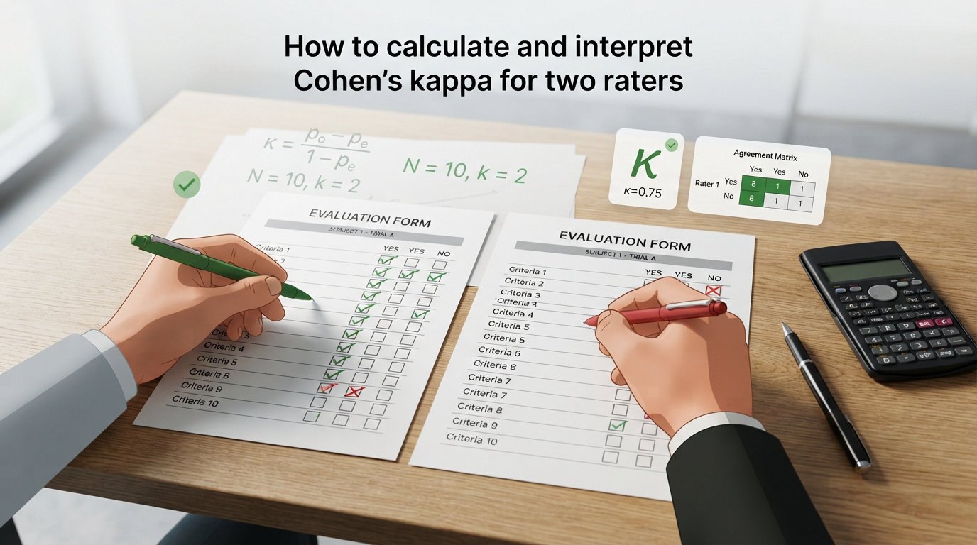
Cohen’s kappa (kappa) is a chance-corrected statistic that measures the level of agreement between two raters who classify items into the same categorical groups. It ranges from -1 (complete disagreement) to +1 (perfect agreement), with 0 indicating no agreement beyond what random chance would produce. Unlike simple percent agreement, Cohen’s kappa accounts for the fact that two raters will agree on some portion of items purely by luck, especially when one category dominates the data.

If you have ever had two colleagues code survey responses, two doctors review the same X-rays, or two annotators label training data for a machine learning model, you have faced the same core question: how do you know they are actually agreeing with each other rather than just guessing the same way? That is exactly the problem Cohen’s kappa solves. Learning how to calculate and interpret Cohen’s kappa for two raters gives you a defensible, publishable metric for inter-rater reliability that holds up in peer review, clinical research, and model evaluation reports.

In this guide, I will walk you through the kappa formula, two fully worked calculation examples (including one with unequal marginal totals), the Landis and Koch interpretation scale, confidence intervals, negative kappa values, weighted kappa, sample size guidance, and the most common pitfalls researchers hit. By the end, you will be able to run a kappa analysis by hand and explain every number in your results section.

What Is Cohen’s Kappa?

Cohen’s kappa is a reliability statistic designed specifically for two raters who each independently classify the same set of items into mutually exclusive categories. Jacob Cohen introduced the coefficient in 1960 as a way to fix a glaring problem with percent agreement: two raters will always agree on some items just by chance, and that chance agreement inflates the apparent consistency between them.

The kappa coefficient strips out that chance component. It tells you how much better your raters are doing than they would if they were both assigning categories at random, governed only by how often each category appears in the dataset. The result is a single number between -1 and +1 that you can report alongside your classification study.

Here is what the ends of the kappa range mean:

• +1 means perfect agreement. The two raters classified every single item the same way.
• 0 means the observed agreement is exactly what you would expect from chance alone. The raters show no real consistency.
• -1 means systematic disagreement. The raters disagree on every item where disagreement is mathematically possible.

In practice, most kappa values in published research land somewhere between 0.2 and 0.9. A kappa of exactly 0 or below is a red flag that your raters are not on the same page, or that your category distribution is so imbalanced that the statistic itself becomes unreliable.

One common source of confusion: Cohen’s kappa applies to nominal data, where categories have no natural order. Think “positive vs negative diagnosis,” “spam vs not spam,” or “red vs blue vs green.” If your categories have a meaningful order (mild, moderate, severe), you are better served by weighted kappa, which I cover later in this guide.

Inter-Rater Reliability vs. Intrarater Reliability

Cohen’s kappa can measure two related but distinct concepts. Inter-rater reliability asks whether two different people classify items the same way. Intrarater reliability asks whether the same person, rating the same items on two different occasions, is consistent with themselves. The math is identical. The difference is entirely in your study design.

When Should You Use Cohen’s Kappa?

You should reach for Cohen’s kappa when all of the following are true:

• You have exactly two raters (for three or more, use Fleiss’ kappa instead).
• Each rater classifies the same set of items into the same set of categories.
• The categories are nominal (unordered) or you are treating them as nominal.
• You want a chance-corrected measure rather than raw percent agreement.

Typical use cases include medical diagnosis agreement studies, human annotator reliability checks for machine learning training data, survey coding consistency, clinical laboratory quality control, and UX research coding reliability.

The Cohen’s Kappa Formula Explained

The kappa formula looks compact, but each piece carries real meaning. Here it is:

kappa = (po – pe) / (1 – pe)

Two quantities drive the entire calculation:

po (observed agreement) is the proportion of items where the two raters chose the same category. You calculate it by adding up the diagonal cells of your contingency table (the cells where both raters agree) and dividing by the total number of items rated.

pe (expected agreement) is the proportion of agreement you would expect if both raters assigned categories randomly, based on how often each rater uses each category overall. You calculate it from the marginal totals of your contingency table.

The numerator (po minus pe) measures how much extra agreement your raters produce beyond chance. The denominator (1 minus pe) is the maximum possible extra agreement, given the marginal distributions. So kappa is essentially a ratio: “how much better than chance did they do, relative to how much better than chance was even possible?”

If po equals pe, kappa is zero. If po equals 1 (perfect agreement) and pe is less than 1, kappa equals 1. If po is less than pe, kappa goes negative.

How to Calculate Cohen’s Kappa Step by Step

Let me walk you through a complete worked example. I will use a medical diagnosis scenario because that is where kappa gets used most heavily in published research.

Example 1: Two Doctors Diagnosing a Condition

Suppose two radiologists, Dr. A and Dr. B, each review 100 mammograms and classify each as either “Positive” (suspicious for malignancy) or “Negative” (no finding). Here are the results in a 2×2 contingency table:

	Dr. B: Positive	Dr. B: Negative	Row Total
Dr. A: Positive	40	10	50
Dr. A: Negative	5	45	50
Column Total	45	55	100

Step 1: Calculate po (observed agreement).

Add the agreement cells (the diagonal): 40 (both positive) + 45 (both negative) = 85. Divide by the total number of items: 85 / 100 = 0.85. So po = 0.85.

Step 2: Calculate pe (expected agreement).

For each cell on the diagonal, multiply the corresponding row total by the column total, then divide by the grand total. Add those up.

For the “both positive” cell: (50 x 45) / 100 = 22.5. For the “both negative” cell: (50 x 55) / 100 = 27.5. Expected agreement count = 22.5 + 27.5 = 50. Divide by 100: pe = 0.50.

Step 3: Plug into the kappa formula.

kappa = (po – pe) / (1 – pe) = (0.85 – 0.50) / (1 – 0.50) = 0.35 / 0.50 = 0.70

A kappa of 0.70 falls in the “substantial agreement” band on the Landis and Koch scale, which I will cover shortly. This is a solid result for a clinical diagnostic agreement study.

Example 2: Unequal Marginal Totals (The Realistic Case)

Most published examples use symmetrical data where both raters choose each category equally often. Real data is rarely that clean. Let me show you what happens when the marginal totals are lopsided.

Two pathologists review 200 tissue samples and classify each as “Normal” or “Abnormal.” Dr. X is conservative and rarely calls something abnormal. Dr. Y is more aggressive. Here are the results:

	Dr. Y: Normal	Dr. Y: Abnormal	Row Total
Dr. X: Normal	150	20	170
Dr. X: Abnormal	5	25	30
Column Total	155	45	200

Step 1: po = (150 + 25) / 200 = 175 / 200 = 0.875. That is 87.5% raw agreement, which sounds excellent.

Step 2: pe = [(170 x 155) / 200 + (30 x 45) / 200] / 200 x 200. Let me simplify. Expected agreement for “both Normal”: (170 x 155) / 200 = 131.75. Expected agreement for “both Abnormal”: (30 x 45) / 200 = 6.75. Total expected agreement count = 138.5. Divide by 200: pe = 0.6925.

Step 3: kappa = (0.875 – 0.6925) / (1 – 0.6925) = 0.1825 / 0.3075 = 0.59

Notice what just happened. The raw percent agreement was 87.5%, which sounds impressive. But kappa is only 0.59 (moderate agreement) because so much of that 87.5% was predictable from chance alone. When one category dominates (85% of samples are “Normal” according to Dr. X), the expected agreement is high, and kappa adjusts accordingly.

This is the single most common surprise researchers encounter. They report 85% agreement, compute kappa, and get a number in the 0.5 range. The kappa is not wrong. It is telling you that much of the apparent agreement was structural, not meaningful.

How to Interpret Cohen’s Kappa Values

The most widely used interpretation scale comes from Landis and Koch (1977). While their thresholds are arbitrary (the authors themselves called them “clearly arbitrary”), the scale has become the de facto standard across healthcare, social science, and machine learning research.

Kappa Value	Level of Agreement	% of Data That Is Reliable
Below 0.00	Poor agreement	Less than 0%
0.01 to 0.20	Slight agreement	1% to 20%
0.21 to 0.40	Fair agreement	21% to 40%
0.41 to 0.60	Moderate agreement	41% to 60%
0.61 to 0.80	Substantial agreement	61% to 80%
0.81 to 1.00	Almost perfect agreement	81% to 100%

The “% of data that is reliable” column comes from the NIH framework popularized by McHugh (2012). It gives an intuitive reading: a kappa of 0.60 means roughly 60% of the rated data is reliably classified, and the remaining 40% is noise.

What Does a Kappa of 0.6 Mean?

A Cohen’s kappa of 0.6 falls at the upper end of “moderate agreement” on the Landis and Koch scale. It means your raters agree substantially more than chance would predict, but there is still meaningful disagreement in the data. For exploratory social science research, 0.6 may be acceptable. For clinical diagnosis where patient safety is at stake, most methodologists recommend a minimum of 0.80 or higher.

What Is Considered Good Inter-Rater Reliability?

The answer depends on your field. In healthcare research, the commonly cited threshold is 0.80 or above (almost perfect agreement), because diagnostic errors carry serious consequences. In social science and survey research, 0.60 is often considered the minimum acceptable level. In machine learning model evaluation against human ground truth labels, kappa above 0.40 is generally considered a meaningful improvement over a random classifier, though you should aim higher.

Healthcare-Specific Thresholds

For clinical and healthcare applications, McHugh (2012) recommends a more conservative reading of the Landis and Koch scale. A kappa below 0.40 in a healthcare context suggests the data collection protocol needs serious revision or retraining. A kappa between 0.40 and 0.60 may be acceptable for exploratory studies but should be treated with caution. Only kappa values above 0.80 should be considered strong enough for clinical decision-making tools.

Cohen’s Kappa vs. Percent Agreement

Percent agreement is the simplest reliability metric: count how often the two raters agree, divide by the total number of items, and report it as a percentage. It is easy to calculate and easy to explain. But it has one fatal flaw that Cohen’s kappa was specifically designed to fix.

Percent agreement does not distinguish between real agreement and chance agreement. If two raters each classify 100 items as “Yes” or “No,” and both raters say “Yes” 95 times, they will agree at least 90% of the time even if they are choosing randomly within those proportions. The 90% figure looks impressive but tells you almost nothing about whether the raters are actually consistent.

Here is a comparison of the two metrics:

Feature	Percent Agreement	Cohen’s Kappa
Corrects for chance	No	Yes
Range	0% to 100%	-1 to +1
Affected by imbalanced data	Inflated by imbalance	Adjusts for imbalance
Interpretation standards	No universal thresholds	Landis and Koch scale
Difficulty to calculate	Very simple	Moderate (requires marginal totals)
Accepted in peer review	Often rejected alone	Widely accepted

Is Cohen’s Kappa Better Than Percent Agreement?

In most research contexts, yes. Cohen’s kappa provides a chance-corrected measure that percent agreement cannot match. However, percent agreement still has a role. When your data has perfectly balanced categories and a large sample, percent agreement and kappa will tell very similar stories. Some researchers recommend reporting both: kappa for the chance-corrected statistic, and percent agreement for intuitive interpretability.

NIH guidance suggests that percent agreement is acceptable as a supplementary metric but should never be the sole reliability measure in a published study. Reviewers in healthcare journals will almost always ask for kappa if you only report percent agreement.

When Is Percent Agreement Actually Sufficient?

Percent agreement works fine when your categories are evenly distributed and you have a large sample. If both raters use each category roughly 50% of the time across hundreds of items, chance agreement is around 50%, and percent agreement above 80% genuinely reflects strong rater consistency. But the moment your data becomes imbalanced (one category dominates), percent agreement becomes unreliable and you need kappa.

What Does a Negative Cohen’s Kappa Mean?

A negative kappa value surprises many researchers, but it is mathematically possible and practically meaningful. Negative kappa occurs when the observed agreement between raters is lower than the agreement you would expect from chance alone.

This can happen for several reasons:

• The raters are systematically disagreeing, perhaps because they are using different diagnostic criteria or interpreting the rating scale differently.
• The categories are poorly defined, so raters interpret them in opposite ways.
• The sample is too small, and random noise is driving the result.
• One rater is reversed in their coding (for example, rating “1” for positive when the other rater rates “1” for negative).

Any kappa at or below zero indicates no reliable agreement. If you encounter a negative kappa, stop and investigate before publishing. Check whether your raters received the same training, whether the category definitions are clear, and whether one rater may have their scale inverted. A coding error is often the culprit.

In published research, a negative kappa is almost always a sign that something is wrong with the data collection process, not just a low level of agreement.

Confidence Intervals and Standard Error of Kappa

A single kappa value is a point estimate. It tells you what the agreement was in your specific sample, but it does not tell you how precise that estimate is. That is where the standard error and confidence interval come in.

The standard error of kappa is calculated using an asymptotic formula that accounts for the number of categories, the sample size, and the marginal distributions. The most commonly used formula (from Fleiss, Levin, and Paik) is:

SE(kappa) = sqrt[ pe(1 – pe) / (n(1 – pe)^2) ]

Where n is the total number of items rated and pe is the expected agreement. The formula gets more complex for multiple categories, but software like R, SPSS, and Python’s scikit-learn handle this automatically.

Once you have the standard error, the 95% confidence interval is:

kappa plus or minus 1.96 x SE(kappa)

Why Confidence Intervals Matter

Reporting kappa without a confidence interval is like reporting a survey result without a margin of error. A kappa of 0.65 with a 95% CI of 0.20 to 1.00 tells a very different story than a kappa of 0.65 with a 95% CI of 0.60 to 0.70. The first is barely reliable. The second is a tight, trustworthy estimate.

Most peer-reviewed journals now require confidence intervals alongside kappa values. If your sample size is small (under 50 items), your confidence interval will be wide, and you should be cautious about drawing strong conclusions.

Example Confidence Interval Calculation

Using Example 1 from earlier (kappa = 0.70, po = 0.85, pe = 0.50, n = 100):

SE(kappa) = sqrt[ 0.50 x 0.50 / (100 x 0.50) ] = sqrt[ 0.25 / 50 ] = sqrt(0.005) = 0.0707

95% CI = 0.70 plus or minus (1.96 x 0.0707) = 0.70 plus or minus 0.139

The 95% confidence interval is 0.561 to 0.839. This range stays entirely within the “moderate to substantial agreement” bands, which gives us confidence in the result.

Cohen’s Kappa vs. Weighted Kappa

Standard Cohen’s kappa treats all disagreements equally. If Rater A says “mild” and Rater B says “severe,” that counts as one disagreement. If Rater A says “mild” and Rater B says “moderate,” that also counts as one disagreement. But in reality, the first pair is a bigger disagreement than the second.

Weighted kappa fixes this by assigning weights to each disagreement based on how far apart the two ratings are. It is designed for ordinal data, where categories have a natural order (mild, moderate, severe, very severe).

Two weighting schemes are commonly used:

• Linear weights penalize disagreements proportionally to their distance. A two-category gap gets twice the penalty of a one-category gap.
• Quadratic weights penalize larger disagreements more heavily. A two-category gap gets four times the penalty of a one-category gap.

Use weighted kappa when your categories are ordered and the distance between categories matters. Use standard Cohen’s kappa when your categories are nominal (unordered) or when you want every disagreement to count the same regardless of “distance.”

If you are working with a 3-point or 5-point Likert-type scale, weighted kappa is almost always the better choice. Treating “slightly disagree vs strongly agree” the same as “slightly disagree vs slightly agree” throws away meaningful information about the magnitude of disagreement.

Limitations and Pitfalls of Cohen’s Kappa

Cohen’s kappa is the most widely used inter-rater reliability statistic, but it is not without problems. Understanding its limitations helps you avoid misinterpreting your results and keeps you from drawing wrong conclusions in your research.

Pitfall 1: The Kappa Paradox (Prevalence Problem)

The most notorious limitation of kappa is the so-called “kappa paradox.” When the prevalence of one category is very high or very low (imbalanced data), kappa can be substantially lower than percent agreement, even when the raters are genuinely consistent. This happens because extreme marginal distributions drive expected agreement (pe) up, which compresses the denominator of the kappa formula and makes kappa artificially small.

In Example 2 above, the raters agreed 87.5% of the time, but kappa was only 0.59. That gap is the kappa paradox in action. It does not mean the raters are unreliable. It means the data distribution is working against the statistic.

Pitfall 2: Kappa Is Sensitive to Sample Size

With small samples, kappa becomes unstable. A kappa calculated from 20 items could swing wildly if you added 10 more items. As a general rule, aim for at least 50 rated items, and preferably 100 or more, before trusting a kappa estimate. Always report the confidence interval so readers can see the precision of your estimate.

Pitfall 3: Kappa Only Works for Two Raters

Cohen’s kappa is strictly defined for two raters. If you have three or more raters, you need Fleiss’ kappa, which generalizes the approach to multiple raters. Some researchers try to work around this by computing pairwise Cohen’s kappa for each pair of raters and averaging them, but this is statistically inferior to using Fleiss’ kappa directly.

Pitfall 4: Maximum Achievable Kappa Is Often Less Than 1

Most textbooks say kappa ranges from -1 to +1. But for any given set of marginal totals, the maximum achievable kappa may be well below 1. If the two raters have very different category distributions (one rater says “Yes” 90% of the time, the other says “Yes” 50% of the time), perfect agreement is mathematically impossible. You should compare your observed kappa to the maximum achievable kappa for your data, not to 1.0.

Kappa vs. Other Reliability Measures

Cohen’s kappa is not the only option. Here is how it compares to the alternatives:

Measure	Number of Raters	Data Type	Key Difference
Cohen’s kappa	Exactly 2	Nominal	Chance-corrected, unweighted
Weighted kappa	Exactly 2	Ordinal	Penalizes larger disagreements more
Fleiss’ kappa	3 or more	Nominal	Generalizes kappa to multiple raters
Krippendorff’s alpha	2 or more	Nominal, ordinal, interval, ratio	Handles missing data and multiple data types
ICC (Intraclass Correlation)	2 or more	Continuous (interval/ratio)	For continuous data, not categorical
Percent agreement	Any	Any	No chance correction

Sample Size Considerations for Reliable Kappa

Sample size directly affects the stability and interpretability of your kappa estimate. There is no single magic number, but several guidelines can help you plan your study.

The most commonly cited minimum is 30 to 50 items rated by each rater. However, this minimum assumes a binary classification with roughly balanced categories. If you have more than two categories, or if your data is highly imbalanced, you need a larger sample.

For reliable confidence intervals, aim for at least 100 items. With 100 items, your confidence interval will be reasonably narrow, and your kappa estimate will not swing dramatically with small changes in the data.

For clinical and healthcare studies where decisions carry real consequences, some methodologists recommend 200 or more items. The reasoning is simple: a wide confidence interval in a clinical context could mean the difference between accepting a diagnostic protocol that is unreliable and rejecting one that is actually solid.

Several factors push your required sample size higher:

• More categories (a 5-category scale needs more items than a binary scale).
• Imbalanced category distributions (if one category appears 90% of the time, you need more items overall).
• Higher target kappa values (distinguishing 0.80 from 0.85 requires more precision than distinguishing 0.40 from 0.45).
• Small expected disagreements (if raters rarely disagree, you need more items to estimate the disagreement rate accurately).

If you are planning a study and want to compute the required sample size for a target kappa and desired confidence interval width, look for a kappa sample size calculator. Several free tools are available online.

Practical Tips for Researchers

After walking through the math and the pitfalls, here are the practical takeaways I have gathered from working with kappa across research projects:

Always report kappa alongside percent agreement. Reviewers and readers want both numbers. Kappa gives the chance-corrected measure. Percent agreement gives the intuitive measure. Together, they paint a complete picture.

Report the confidence interval every time. A kappa of 0.65 without a CI is incomplete. A kappa of 0.65 with a 95% CI of 0.45 to 0.85 is honest and informative.

If your kappa is lower than expected, check the marginal distributions before blaming your raters. The kappa paradox is real. Sometimes the data distribution is the problem, not the raters.

Train your raters before collecting data. Kappa is a measure of consistency, not correctness. Two raters can be perfectly consistent and both wrong. Training ensures they are consistently correct.

Pilot your rating instrument on a small sample first. Compute kappa on the pilot data. If kappa is below 0.40, revise your category definitions, retrain your raters, and pilot again before committing to a full study.

Frequently Asked Questions

Conclusion

Knowing how to calculate and interpret Cohen’s kappa for two raters gives you a publishable, peer-review-ready measure of inter-rater reliability that goes far beyond what simple percent agreement can tell you. The formula kappa = (po – pe) / (1 – pe) strips out chance agreement and reveals the true level of consistency between your raters.

Remember the key takeaways: always report kappa with a confidence interval, watch for the kappa paradox when your data is imbalanced, use weighted kappa for ordinal scales, switch to Fleiss’ kappa for three or more raters, and pilot your rating instrument before committing to a full study. With these tools in hand, you are ready to design a reliability study that holds up under review and gives your readers confidence in your data quality.

Start by building your contingency table from a pilot sample of 30 to 50 items, calculate po and pe by hand using the steps in this guide, and verify your results against a software tool like R, Python, or SPSS. Once your manual calculation matches the software output, you will have the confidence to run kappa analyses on any dataset.