
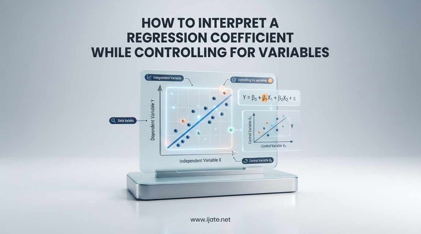
If you have ever read a research paper that said “we controlled for age, income, and education,” you have run into one of the most misunderstood ideas in statistics. Learning how to interpret a regression coefficient while controlling for other variables is the skill that separates people who can run a model from people who can actually explain what the model means.
I have spent years teaching this concept to students, analysts, and researchers. Almost everyone gets the mechanics of running a regression in software. Far fewer people can confidently say what a coefficient represents once other predictors enter the model. The phrase “holding other variables constant” gets tossed around, but few resources explain what it actually means in plain language.
This guide fixes that gap. We will walk through what “controlling” really means, how the math makes it happen, and how you should read a coefficient table once control variables are included. We will also cover the cases where controlling for a variable is the wrong move, which is something almost no competing resource discusses.
By the end, you will have a clear mental model for interpreting any multiple regression coefficient, a practical checklist for your own work, and the confidence to explain your results to stakeholders without falling back on vague phrases. Whether you work in R, Python, SPSS, Stata, or Excel, the interpretation principles here apply universally.
Table of Contents
Quick Answer: The 60-Second Definition
A regression coefficient, when controlling for other variables, represents the estimated average change in the dependent variable for a one-unit increase in that specific independent variable, while holding all other predictors in the model constant at their current values. It isolates the unique contribution of that single predictor after removing the overlapping influence of every other variable in the equation.
Think of it this way. Without control variables, a coefficient tells you the total association between a predictor and the outcome, including any shared variance with other factors. With controls in place, the coefficient tells you only the part of that relationship that belongs uniquely to that predictor. That is the difference between a simple regression slope and a partial regression coefficient.
This distinction matters because real-world variables are correlated. Income correlates with education, age correlates with experience, and body weight correlates with height. If you ignore those overlaps, your coefficients will absorb effects that belong to other variables, and your interpretation will be misleading.
What Does It Mean to Control for a Variable in Regression?
Controlling for a variable means accounting for its influence so that the relationship between your main variable of interest and the outcome is not contaminated by that factor. In a regression context, you accomplish this by including the control variable as an additional predictor in the model.
Imagine you are studying the relationship between hours studied and exam scores. Without any controls, you might find that students who study more score higher. But what if those students also sleep more, attend better schools, or have stronger prior knowledge? Any of those factors could inflate the apparent benefit of studying.
By adding those factors as control variables in your regression, you statistically separate the effect of studying from the effects of sleep, school quality, and prior knowledge. The coefficient on hours studied then reflects only the portion of the exam-score relationship that is uniquely tied to study time.
There are several ways to control for variables, but regression is by far the most common. Other approaches include stratification (splitting your data into subgroups), matching (pairing observations with similar characteristics), weighting, and randomization in experimental designs. Each method achieves the same goal through different mechanics, but multiple regression is the workhorse because it handles many control variables simultaneously and works with continuous predictors.
The phrase “controlling for” is synonymous with “holding constant,” “adjusting for,” “accounting for,” and the Latin term “ceteris paribus” (all else equal). You will see all of these in textbooks and published papers. They all describe the same statistical operation: isolating one variable’s effect by mathematically removing the influence of others.
One common confusion is the idea that the software literally fixes control variables at a single value. It does not. The phrase “holding other variables constant” is an interpretive shorthand, not a literal description of what the algorithm does. The math works by removing shared variance, not by clamping variables to specific numbers. We will get into the exact mechanics later in this article.
How to Interpret a Regression Coefficient While Controlling for Other Variables
Interpreting a controlled regression coefficient comes down to one sentence template that you can apply to any output table. Once you memorize it and practice it a few times, reading coefficient tables becomes second nature.
The Interpretation Template
For a one-unit increase in [predictor], the dependent variable changes by [coefficient value] units, on average, while holding all other variables in the model constant.
That is the entire interpretation in one line. Every word matters. “One-unit increase” defines the comparison the model is making. “On average” reminds you that regression describes expected or mean relationships, not guarantees for individuals. “Holding all other variables constant” is the controlling language that separates this from a simple regression slope.
A Concrete Example
Suppose you run a multiple regression predicting salary from years of experience, education level, and age. Your software outputs a coefficient of 3,200 for years of experience. The correct interpretation is: for each additional year of experience, salary increases by 3,200 dollars on average, holding education level and age constant.
Notice what you are not saying. You are not claiming that every extra year of experience adds exactly 3,200 dollars to every person’s salary. You are not ignoring education and age. You are saying that after the model accounts for the salary effects of education and age, the remaining unique contribution of an extra year of experience is 3,200 dollars on average.
Step-by-Step Interpretation Process
Follow these steps every time you read a coefficient from a multiple regression output.
Step 1: Identify the dependent variable (the outcome your model predicts). Every coefficient in the table is expressed in units of this variable. If the dependent variable is measured in dollars, coefficients are in dollars.
Step 2: Identify the specific predictor whose coefficient you want to interpret. Look only at that row of the output table.
Step 3: Note the units of that predictor. A coefficient of 2.5 means something very different if the predictor is measured in single units versus thousands. The interpretation always references a one-unit increase in whatever unit the predictor uses.
Step 4: Read the coefficient value and apply the template. Insert the predictor name, the unit of the dependent variable, and the coefficient value into the sentence structure above.
Step 5: List the control variables by name. Saying “holding all other variables constant” is correct, but naming the specific controls makes your interpretation clearer and more credible to readers.
Step 6: Check the sign. A positive coefficient means the outcome increases as the predictor increases. A negative coefficient means the outcome decreases. A coefficient near zero means the predictor has essentially no unique relationship with the outcome after controlling for other variables.
Step 7: Check statistical significance before drawing strong conclusions. We cover p-values and confidence intervals in detail later in this guide.
What the Coefficient Does Not Tell You
A controlled coefficient tells you about association, not necessarily causation. Even after controlling for many variables, there may be unmeasured confounders that bias the estimate. The coefficient is also specific to the set of variables in your model. Add or remove a variable, and the coefficient can change.
The coefficient also does not tell you about the practical importance of the effect. A coefficient can be statistically significant but trivially small in real-world terms. Always pair the coefficient value with domain knowledge to judge whether the effect size matters for your decision-making.
A Worked Example: Why Controlling Changes Your Results
The best way to understand why controlling matters is to see a coefficient change before and after you add a control variable. Let us work through a simple example inspired by a classic scenario discussed on statistics forums.
The Setup
Imagine you are analyzing data from 200 employees. You want to know whether having a mentor increases employee productivity, measured as completed projects per quarter. You start with a simple regression of productivity on a binary mentor variable (1 if the employee has a mentor, 0 otherwise).
The simple regression returns a coefficient of 4.0 for the mentor variable. Employees with mentors complete 4.0 more projects per quarter than employees without mentors. That sounds impressive, but you suspect that employees with mentors also tend to have more prior experience.
Adding the Control Variable
You add years of prior experience as a control variable and rerun the regression. Now the mentor coefficient drops to 1.2. The coefficient for prior experience is 0.8, meaning each year of prior experience adds 0.8 projects per quarter on average, holding mentor status constant.
What happened? The original 4.0-project gap was inflated because mentorship and experience were correlated. Employees with mentors also tended to be more experienced, and that experience was driving part of the productivity difference. Once you controlled for experience, the unique effect of having a mentor shrank to 1.2 projects.
The Stratification Way to See the Same Thing
You can arrive at the same conclusion by stratifying your data. Split employees into groups based on years of prior experience: low experience, medium experience, and high experience. Within each group, compare the productivity of employees with and without mentors.
If mentorship has a true unique effect, you should see a consistent gap within each experience stratum. Averaging those within-stratum gaps (weighted by group size) gives you roughly the same estimate as the multiple regression coefficient. This is the intuitive bridge between stratification and regression that many learners find illuminating.
Why the Coefficient Dropped
The coefficient dropped because prior experience was a confounding variable. It was correlated with both the predictor (mentorship) and the outcome (productivity). Confounders inflate or deflate coefficients when left out of the model. Controlling for them removes that distortion.
This is exactly why published research papers always list their control variables. Without knowing the controls, you cannot judge whether the reported coefficients reflect real unique effects or are contaminated by omitted variables. The same logic applies whether you are studying drug efficacy, marketing ROI, or educational interventions.
It is also possible for a coefficient to increase after adding a control, not just decrease. This happens when a suppressor variable is at play, where the control variable masks the true relationship. Either way, the takeaway is the same: adding controls can substantially change coefficients, and that change is the entire point of running a multiple regression instead of a simple one.
How Multiple Regression Controls Mathematically (Partialling Out)
At this point you might be wondering how the software actually does the controlling. It does not literally freeze variables at fixed values. Instead, it uses a process called partialling out, which is grounded in the Frisch-Waugh-Lovell theorem. Understanding this process removes the mystery behind the phrase “holding other variables constant.”
The Partialling-Out Process in Plain Terms
Partialling out works in three conceptual steps for each predictor. First, the algorithm regresses your main predictor of interest on all the control variables and saves the residuals. Those residuals represent the part of your main predictor that cannot be explained by the controls. Second, it regresses the dependent variable on the same controls and saves those residuals. Third, it relates the two sets of residuals to each other.
In other words, the coefficient on your main predictor is estimated from what is left over after the control variables have explained everything they can about both the predictor and the outcome. The control variables “eat” their shared variance first, and the remaining unique variance is what your coefficient captures.
The Frisch-Waugh-Lovell Theorem
The Frisch-Waugh-Lovell theorem, developed by economists Ragnar Frisch and Frederick Waugh in 1933 and extended by Michael Lovell in 1963, proves that the coefficient you get from a full multiple regression is identical to the coefficient you get from this three-step partialling-out procedure. The theorem holds for ordinary least squares (OLS) regression and is one of the most elegant results in econometrics.
This theorem is why we can confidently say that a multiple regression coefficient represents the unique effect of a variable after removing the influence of all other variables in the model. The math guarantees it. When you report a controlled coefficient, you are reporting an estimate built purely from residualized variance.
A Geometric Way to Think About It
If you prefer visual thinking, consider the geometric interpretation. In multiple regression, each variable can be represented as a vector in an n-dimensional space (one dimension per observation). The control variables define a subspace. Partialling out means projecting your main predictor and your outcome onto the part of the space that is perpendicular to the control subspace.
The coefficient is then the slope of the relationship between those two projected, perpendicular components. This is why the procedure is sometimes described as “orthogonalizing” a variable with respect to the controls. The geometry is not necessary for practical interpretation, but it confirms that “holding constant” is a real mathematical operation, not a hand-wavy metaphor.
Why This Matters for Interpretation
Understanding partialling out prevents several common mistakes. First, it explains why adding a highly correlated variable can cause coefficients to swing wildly or flip signs. The two variables are fighting over the same shared variance, and partialling out leaves very little unique variance to estimate. Second, it explains why a variable that is significant in simple regression can become insignificant after controls. Its apparent effect was largely shared with other predictors, leaving little unique contribution.
Third, it clarifies why multicollinearity is a problem. When control variables are highly correlated with your main predictor, the residualized unique component is small and estimated imprecisely, inflating standard errors and destabilizing the coefficient. We will discuss multicollinearity detection in the assumptions section.
Finally, partialling out reminds you that a coefficient is always defined relative to the specific set of variables in the model. Change the controls, and you change what is being partialled out, which changes the coefficient. There is no single “true” coefficient for a variable independent of model specification.
Unstandardized vs Standardized Coefficients
When you read regression output, most software reports two versions of each coefficient: unstandardized and standardized. Knowing when to interpret which one is essential, and mixing them up is a common source of miscommunication.
Unstandardized Coefficients
Unstandardized coefficients are the default. They are expressed in the original units of the predictor and the dependent variable. A coefficient of 3,200 for years of experience means 3,200 dollars per year, full stop. You use unstandardized coefficients when you want to communicate effects in meaningful, real-world units or when you need to make predictions from the model.
Unstandardized coefficients are also what you report when your audience cares about the practical magnitude of an effect. Stakeholders understand “3,200 dollars per year.” They do not understand “0.4 standard deviations per standard deviation” without a lot of context.
Standardized Coefficients (Beta Weights)
Standardized coefficients, often called beta weights, are expressed in standard deviation units. Both the predictor and the dependent variable are converted to z-scores before the regression is estimated. A standardized coefficient of 0.4 means that a one-standard-deviation increase in the predictor is associated with a 0.4-standard-deviation increase in the outcome, holding other variables constant.
Standardized coefficients are useful when you want to compare the relative importance of predictors measured on different scales. If your model includes income in dollars, age in years, and education in years, the unstandardized coefficients are not directly comparable because the units differ. Standardized coefficients put everyone on the same footing.
When to Use Which
Use unstandardized coefficients for prediction, communication with non-technical audiences, and any situation where real-world units matter. Use standardized coefficients for comparing the relative strength of predictors within the same model or for published academic work where effect-size comparison across variables is the goal.
Never report only standardized coefficients without also providing the unstandardized versions. Reviewers and readers need both to fully understand the model. Also be aware that standardized coefficients are sensitive to the sample’s variability. A beta weight of 0.4 in one sample may not translate to the same real-world effect in a different population with a different standard deviation.
Some researchers caution against using standardized coefficients for causal claims because the standard deviation is a sample-specific quantity. If you are building a model intended to generalize across populations, unstandardized coefficients are more stable and interpretable across contexts.
Reading the Regression Output (p-values, Confidence Intervals, R-squared)
Interpreting the coefficient value is only half the job. You also need to read the supporting statistics that tell you whether the coefficient is reliable and how well the model fits. The three most important pieces are the p-value, the confidence interval, and R-squared.
P-values and Statistical Significance
The p-value attached to each coefficient answers a specific question: if the true coefficient were zero (meaning no real relationship after controlling for other variables), how likely is it that you would observe a coefficient at least this large by chance alone? A p-value below 0.05 means that probability is below 5%, which most fields treat as the threshold for statistical significance.
A significant coefficient is one where you can confidently rule out chance as the explanation for the observed relationship. A non-significant coefficient means the data do not provide enough evidence to rule out zero, given the controls in the model. It does not prove the effect is zero, only that your sample cannot distinguish it from zero.
Confidence Intervals
The 95% confidence interval gives you a range of plausible values for the true coefficient. If the interval runs from 800 to 5,600, you can say with reasonable confidence that the true effect of a one-unit increase in the predictor lies somewhere in that range, holding other variables constant.
Always check whether the confidence interval crosses zero. If it does, the coefficient is not statistically significant at the 0.05 level. Confidence intervals are more informative than p-values alone because they show the precision of the estimate, not just whether it clears an arbitrary threshold.
R-squared and Adjusted R-squared
R-squared tells you the proportion of variance in the dependent variable that your model explains. An R-squared of 0.9 means that 90% of the variation in the outcome is accounted for by the predictors in your model. The remaining 10% is unexplained variation due to omitted factors or random noise.
Be cautious with very high R-squared values. A value above 0.9 can indicate a strong model, but it can also signal overfitting, especially if you have many predictors relative to your sample size. Adjusted R-squared penalizes the addition of irrelevant predictors and is a better metric when comparing models with different numbers of control variables.
R-squared tells you about model fit, not about individual coefficient interpretation. A model can have a high R-squared and still contain individual coefficients that are not significant, or a model can have a low R-squared and still contain coefficients that are highly significant. Read the two pieces of information separately.
Key Assumptions and Common Pitfalls
The interpretation of a controlled regression coefficient is only valid if the underlying assumptions of OLS regression are reasonably met. Violating these assumptions can bias coefficients, inflate or shrink standard errors, and render your interpretation meaningless.
Linearity
OLS regression assumes a linear relationship between each predictor and the outcome. If the true relationship is curved, the linear coefficient will be a misleading average that does not represent the effect accurately. Always inspect residual plots and consider transformations or polynomial terms if nonlinearity is present.
Homoscedasticity
Homoscedasticity means the variance of residuals is constant across all levels of the predictors. If variance changes (heteroscedasticity), standard errors are unreliable, which means p-values and confidence intervals cannot be trusted. Use residual-versus-fitted plots to check, and apply robust standard errors if the assumption is violated.
Multicollinearity
Multicollinearity occurs when two or more predictors are highly correlated with each other. It inflates standard errors, makes coefficients unstable, and can cause coefficients to flip signs when control variables are added or removed. Detect it using the variance inflation factor (VIF), where values above 5 or 10 indicate problematic collinearity.
If multicollinearity is severe, consider dropping one of the correlated variables, combining them into an index, or using a regularization technique like ridge regression. Just remember that removing a variable changes the partialling-out process and changes every remaining coefficient in the model.
Residual Confounding
Even with control variables, you can never fully rule out confounding from unmeasured factors. Residual confounding is the lingering bias from variables you did not or could not include in the model. It is the single biggest threat to causal interpretation of regression coefficients in observational studies.
Be transparent about which variables you controlled for and which important ones were unavailable. A coefficient from an observational regression is best described as an adjusted association, not a definitive causal effect, unless you have a strong design (randomization, natural experiment, or a validated instrumental variable).
Normality of Residuals
OLS regression assumes residuals are normally distributed. This matters most for small samples. With large samples (typically above 30 observations per predictor), the central limit theorem makes coefficient estimates approximately normal even if residuals are not perfectly so. Check normality with a Q-Q plot or a Shapiro-Wilk test, but do not over-interpret minor deviations in large samples.
When You Should NOT Control for a Variable
Most guidance on regression emphasizes which variables to include. Equally important is knowing which variables to leave out. Including the wrong control variable can distort your coefficient of interest as badly as omitting a confounder. This is a topic almost no competing resource covers, and it is critical for sound interpretation.
Do Not Control for Mediators
A mediator is a variable that lies on the causal pathway between your predictor and the outcome. If education affects income partly because education increases job skills, and job skills increase income, then job skills are a mediator. Controlling for job skills would block part of the effect you are trying to measure, shrinking the coefficient on education and giving you a misleadingly narrow estimate.
Decide whether you want the total effect of your predictor or the direct effect net of mediators. Most policy and business questions call for the total effect, which means you should not control for mediators. Reserve mediator controls for specific mediation-analysis frameworks designed for that purpose.
Do Not Control for Colliders
A collider is a variable that is caused by both your predictor and the outcome (or by their common causes). Controlling for a collider opens a backdoor path that introduces selection bias into your coefficient. The classic example is hospital admission being a collider between many diseases and their outcomes. Conditioning on hospital admission can create a spurious negative association between conditions.
Collider bias is subtle and counterintuitive. If you are unsure whether a variable is a confounder or a collider, draw a directed acyclic graph (DAG) showing your assumptions about causal direction. If arrows flow into the variable from both your predictor and the outcome, it is a collider and should be left out of the model.
Do Not Over-Control
Overcontrol means including so many control variables that the model loses meaningful variance to estimate from. This often happens when researchers add every available variable to a model in the hope of being thorough. The result is unstable coefficients, inflated standard errors, and estimates that no longer reflect the question of interest.
Choose controls based on theory and prior evidence, not on data availability. A smaller, well-justified set of controls produces more interpretable coefficients than a sprawling model packed with marginal adjustments.
FAQs
How do you interpret the coefficients of a regression?
A regression coefficient represents the estimated average change in the dependent variable for a one-unit increase in that independent variable, while holding all other predictors in the model constant. For example, a coefficient of 3,200 for years of experience means each additional year adds 3,200 dollars to salary on average, assuming education and age stay the same.
How to control for other variables in regression?
To control for other variables in regression, include them as additional independent variables in your model alongside your main predictor of interest. The regression algorithm will estimate each coefficient using the partialling-out process, which removes the shared variance between predictors and isolates the unique effect of each one.
What does a R-squared value of 0.9 mean?
An R-squared value of 0.9 means that 90% of the variation in the dependent variable is explained by the independent variables in your model. The remaining 10% is unexplained variation from omitted factors or random noise. Values above 0.9 may also signal overfitting, especially with many predictors relative to sample size.
How to tell if a regression coefficient is significant?
A regression coefficient is statistically significant if its p-value is below your threshold (typically 0.05) or if its 95% confidence interval excludes zero. A p-value below 0.05 means there is less than a 5% chance of observing a coefficient this large if the true effect were zero.
Why do regression coefficients change when you add control variables?
Coefficients change because adding a control variable changes the partialling-out process. The new control absorbs some of the shared variance between your main predictor and the outcome, leaving a different amount of unique variance for your coefficient to capture. This is why the same predictor can have very different coefficients across model specifications.
Conclusion: Your Interpretation Checklist
Knowing how to interpret a regression coefficient while controlling for other variables is a foundational skill for anyone working with data. The interpretation always follows the same template: a one-unit increase in the predictor produces a coefficient-sized change in the outcome, on average, while holding all other variables constant.
Use this checklist each time you read or report a controlled coefficient. Identify the dependent variable and its units. Identify the predictor and its units. Apply the interpretation template with the coefficient value. Name the specific control variables you are holding constant. Check the sign, p-value, and confidence interval. Verify the model assumptions are met. Confirm you are not controlling for mediators or colliders. State clearly whether you are claiming association or causation.
If you internalize one idea from this guide, let it be this. A controlled coefficient is not the total relationship between a variable and an outcome. It is the unique contribution that remains after every other variable in the model has taken its share of the explanation. That distinction is the heart of multiple regression, and it is what makes the technique so powerful for separating signal from noise in real-world data.