
If you have ever run an ANOVA and stared at the output wondering what those eta-squared values actually mean, you are in the right place. Knowing how to interpret eta-squared and partial eta-squared is one of the most useful skills for anyone working with statistical analyses. These two effect size measures tell you not just whether your results are statistically significant, but how much your independent variable actually matters.
Many researchers and students get tripped up here because these two measures look similar but behave differently depending on your study design. I have spent years working through ANOVA outputs in SPSS, R, and JASP, and the confusion around these statistics comes up constantly on forums like r/AskStatistics and r/statistics. The good news is that once you understand what each denominator represents, everything clicks into place.
In this guide, I will walk you through what each measure means, how to calculate both from real ANOVA data, when to use which one, and how to apply Cohen’s interpretation thresholds. I will also flag the common SPSS labeling issue that trips up even experienced researchers.
Table of Contents
What Is Eta Squared?
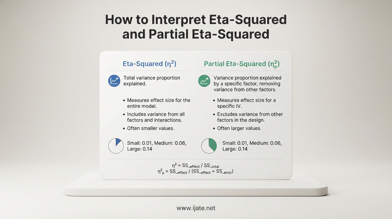
Eta squared (written as η2) is a measure of effect size that represents the proportion of total variance in your dependent variable that is explained by an independent variable. In plain terms, it answers the question: out of all the variation in your data, how much can be attributed to the group differences you are testing?
The formula is straightforward:
η2 = SSeffect / SStotal
Here, SSeffect is the sum of squares for the factor you are examining, and SStotal is the total sum of squares across all sources of variation in your data. The result is always between 0 and 1, and you can express it as either a decimal or a percentage. An eta squared of 0.15 means that 15% of the total variability in your outcome variable is accounted for by group membership.
One thing I always emphasize is that eta squared uses the total sum of squares as its denominator. That includes variance from every source in your study, not just the effect you are looking at. This matters a lot in factorial designs, as we will see shortly.
What Is Partial Eta Squared?
Partial eta squared (ηp2) measures the proportion of variance explained by an independent variable, excluding variance accounted for by other factors in the model. It isolates the specific effect you are examining by removing the influence of other independent variables.
The formula changes the denominator compared to eta squared:
ηp2 = SSeffect / (SSeffect + SSerror)
Instead of dividing by the total sum of squares, partial eta squared divides by the sum of squares for that specific effect plus the error term. This means the denominator only includes variance relevant to the effect being measured, plus unexplained variance. Everything else gets removed from the picture.
Because the denominator is smaller (it excludes other effects), partial eta squared values are almost always equal to or larger than eta squared values for the same effect. The exception is one-way ANOVA, where the two measures produce identical results.
Partial eta squared is the default effect size reported by SPSS for most ANOVA procedures, which is why so many researchers encounter it first. It is particularly useful in factorial designs where you have multiple independent variables and want to understand the unique contribution of each one.
How to Interpret Eta-Squared and Partial Eta-Squared: The Key Difference
The core difference comes down to the denominator. Eta squared divides by the total variance in the model, while partial eta squared divides by only the variance from that specific effect plus error. This single difference changes everything about how you should think about and compare the values.
In a one-way ANOVA with a single independent variable, eta squared and partial eta squared are mathematically identical. There is only one effect, so SStotal equals SSeffect + SSerror, and both formulas reduce to the same thing. I have seen many students realize this and suddenly understand why their numbers matched across different software outputs.
In a factorial ANOVA, the two measures diverge. Suppose you have two independent variables, A and B, plus their interaction AxB. The total sum of squares includes variance from A, B, AxB, and error. When you calculate eta squared for factor A, you divide SSA by SStotal, which includes variance from B and the interaction. Partial eta squared for factor A divides SSA by only SSA + SSerror, removing the variance from B and the interaction entirely.
This means partial eta squared will typically give you a larger value for the same effect in a factorial design. It is not that the effect got bigger, it is that the denominator shrank. Both numbers are correct, but they answer slightly different questions.
I always recommend being explicit about which one you report. Writing “partial eta squared = .14” is far better than just saying “effect size = .14” and leaving the reader to guess.
Cohen’s Interpretation Guidelines
The most widely used benchmarks for interpreting eta squared values come from Jacob Cohen’s foundational work. These thresholds provide a rough guide for classifying effects as small, medium, or large.
For eta squared, Cohen’s guidelines are:
- Small effect: η2 = 0.01 (1% of variance explained)
- Medium effect: η2 = 0.06 (6% of variance explained)
- Large effect: η2 = 0.14 (14% of variance explained)
The same thresholds apply to partial eta squared, and this is where I see a lot of confusion on statistics forums. Many researchers worry when their partial eta squared hits 0.14 in a factorial design, thinking the effect is unusually large. But because partial eta squared uses a smaller denominator, it naturally produces larger values. Reaching the “large” threshold with partial eta squared does not necessarily mean your effect is enormous in an absolute sense.
It is worth noting that Cohen himself described these benchmarks as rough rules of thumb, not rigid cutoffs. The appropriate magnitude depends heavily on your field. In social sciences and education research, effects of 0.01 to 0.06 are common and meaningful. In controlled laboratory experiments or physics research, much larger effects might be expected.
I also want to connect this to Cohen’s f, another popular effect size measure for ANOVA. The relationship is: f = sqrt(η2 / (1 – η2)). Cohen’s f thresholds are small = 0.10, medium = 0.25, large = 0.40, and they map directly onto the eta squared values above.
Step-by-Step Calculation Example With Real Numbers
Let me walk through a concrete example so you can see exactly how both measures work. Suppose we have a 2×2 factorial ANOVA examining how teaching method (factor A: lecture vs. interactive) and class size (factor B: small vs. large) affect test scores.
Here are the sum of squares from our ANOVA table:
- SSA (teaching method) = 180
- SSB (class size) = 120
- SSAxB (interaction) = 60
- SSerror = 640
- SStotal = 1000
Calculating eta squared for factor A:
η2A = SSA / SStotal = 180 / 1000 = 0.18
This tells us that teaching method accounts for 18% of the total variance in test scores. Using Cohen’s guidelines, that qualifies as a large effect.
Calculating partial eta squared for factor A:
ηp2A = SSA / (SSA + SSerror) = 180 / (180 + 640) = 180 / 820 = 0.2195
So partial eta squared for teaching method is approximately 0.22, compared to eta squared of 0.18. The partial version is larger because it excludes the variance from class size and the interaction. It says that of the variance not explained by other factors, teaching method accounts for about 22%.
Let us do the same for factor B (class size):
η2B = 120 / 1000 = 0.12 (medium-to-large effect)
ηp2B = 120 / (120 + 640) = 120 / 760 = 0.158 (large effect by Cohen’s thresholds)
Notice how the same data produces noticeably different values depending on which measure you use. Both are correct descriptions of the data from different perspectives.
For the interaction effect:
η2AxB = 60 / 1000 = 0.06 (medium effect)
ηp2AxB = 60 / (60 + 640) = 60 / 700 = 0.086 (still in the medium range)
This example illustrates why you should never compare eta squared values from one study with partial eta squared values from another. The numbers are not on the same scale in factorial designs.
When to Use Eta Squared vs Partial Eta Squared
Choosing the right measure depends on your study design and what you want to communicate. Here is the decision framework I use.
Use eta squared when: you want to describe the proportion of total variance explained by an effect, especially in one-way ANOVA. It is also preferable when you want to compare effect sizes across studies with different designs, because it is based on total variance.
Use partial eta squared when: you are working with factorial ANOVA, repeated measures ANOVA, or MANOVA, and you want to isolate the unique contribution of a specific factor. It is also the standard output in SPSS, making it the most commonly reported measure in published research.
The decision matters most in multifactor designs. In a 2x3x2 ANOVA with three main effects and multiple interactions, eta squared values for each effect will be relatively small because SStotal includes variance from all other factors. Partial eta squared gives each factor its own stage, producing values that better reflect the isolated impact of that variable.
SPSS warning: SPSS labels its default ANOVA output effect size as “Partial Eta Squared,” but for one-way ANOVA, this is mathematically identical to eta squared. If you are running a one-way ANOVA in SPSS, you can report the value as either eta squared or partial eta squared. They are the same number. The confusion arises when researchers assume they are different and try to convert between them unnecessarily.
One more consideration: if you plan to compute a power analysis for future studies using software like G*Power, that software typically uses partial eta squared or Cohen’s f. Make sure you are using the right input for the tool.
How to Report Effect Sizes in APA Format
Reporting effect sizes properly matters for transparency and reproducibility. APA style requires effect sizes alongside significance tests so readers can evaluate practical importance, not just statistical significance.
Here is the standard APA format for reporting these measures:
“There was a significant main effect of teaching method on test scores, F(1, 96) = 27.00, p < .001, η2 = .18.”
For partial eta squared, the format is nearly identical:
“There was a significant main effect of teaching method on test scores, F(1, 96) = 27.00, p < .001, ηp2 = .22.”
Always specify which measure you are reporting. Use the subscript p notation for partial eta squared. Include the F-statistic, degrees of freedom, p-value, and effect size together in the same statement so readers have the complete picture.
If you report both measures in the same paper, state your choice clearly in the methods section and explain why you chose it for your design.
Common Mistakes and Misinterpretations
Several errors come up repeatedly in student work, published papers, and forum questions. Let me address the most common ones.
Mistake 1: Comparing eta squared from one study with partial eta squared from another. These are not directly comparable in factorial designs. When reviewing literature, check which measure each study reported before drawing conclusions about relative effect magnitudes.
Mistake 2: Assuming partial eta squared can never exceed 1. In most standard ANOVA designs, partial eta squared stays between 0 and 1. However, in certain repeated measures designs with specific covariance structures, values slightly above 1 can theoretically occur. If you see this, check your data and analysis setup.
Mistake 3: Treating Cohen’s thresholds as strict rules. These are guidelines, not law. A partial eta squared of 0.055 is not fundamentally different from 0.06. Report the actual value and interpret it in the context of your field and research question.
Mistake 4: Forgetting that partial eta squared depends on what other factors are in the model. Adding or removing a factor changes the partial eta squared for the remaining factors because the error term shifts. Eta squared, being based on total variance, is more stable across model changes.
Mistake 5: Confusing statistical significance with practical significance. A tiny p-value with a small effect size means you have a real but weak effect. Always report and discuss effect sizes alongside p-values so your readers understand both the reliability and magnitude of your findings.
Frequently Asked Questions
What is the difference between eta squared and partial eta squared?
Eta squared divides the effect sum of squares by the total sum of squares, measuring the proportion of total variance explained. Partial eta squared divides the effect sum of squares by the effect plus error sum of squares, isolating the variance from that specific effect. In one-way ANOVA, the two are identical. In factorial ANOVA, partial eta squared is typically larger because it excludes variance from other factors.
How do you interpret eta squared effect size?
Use Cohen’s guidelines: values of 0.01 indicate a small effect, 0.06 a medium effect, and 0.14 a large effect. These thresholds apply to both eta squared and partial eta squared, though partial eta squared values tend to be larger in factorial designs. Always interpret the value in the context of your research field.
What is partial eta squared in ANOVA?
Partial eta squared is an effect size measure in ANOVA that represents the proportion of variance explained by a specific independent variable, excluding variance accounted for by other independent variables in the model. It is calculated as the effect sum of squares divided by the effect sum of squares plus the error sum of squares.
What are the rules of thumb for interpreting eta squared values?
Cohen’s guidelines classify eta squared values as small at 0.01, medium at 0.06, and large at 0.14. These correspond to 1%, 6%, and 14% of variance explained respectively. The same thresholds apply to partial eta squared, though field-specific expectations may vary.
How do you calculate partial eta squared?
Divide the sum of squares for the effect by the sum of squares for the effect plus the error sum of squares. The formula is: partial eta squared = SS_effect / (SS_effect + SS_error). You can find these values directly in your ANOVA summary table from SPSS, R, or any statistical software.
Conclusion
Understanding how to interpret eta-squared and partial eta-squared gives you a much richer picture of your ANOVA results than p-values alone. Eta squared tells you what proportion of total variance your effect explains, while partial eta squared isolates your effect from other factors in the model.
Remember that the two are identical in one-way ANOVA but diverge in factorial designs. Always specify which measure you are reporting, apply Cohen’s thresholds as guidelines rather than rigid rules, and interpret your values in the context of your specific field. With these tools, you can confidently communicate not just whether your results are significant, but how much they actually matter.
Next time you open an ANOVA output table, take a moment to identify which effect size your software reported and what question it is really answering. That simple habit will make your statistical interpretations sharper and your research more transparent.