How to Run an A Priori Power Analysis in G*Power? (September 2026 Guide)

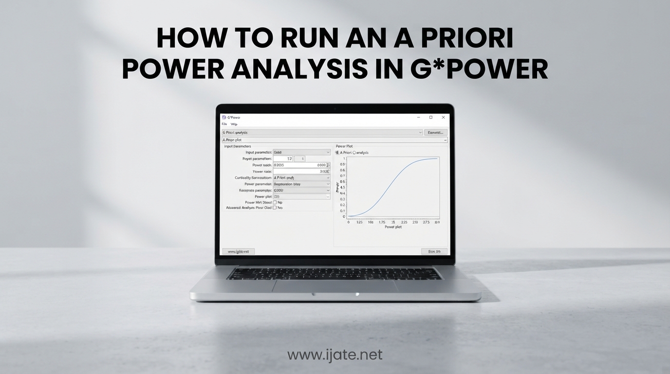
Learning how to run an a priori power analysis in G*Power is one of the most practical skills a researcher can pick up. In short: open G*Power, set Test family to the family matching your test (for example, t tests), set Statistical test to your specific test (for example, Means: Difference between two independent means), choose Type of power analysis: A priori: Compute required sample size, enter an effect size of 0.5, an alpha of 0.05, and a power of 0.80, then click Calculate. For that standard independent samples t-test setup, G*Power returns 64 participants per group, or 128 total.

In this guide, I will walk you through every parameter, every menu, and every common test type. I will also share the mistakes I see researchers make on Reddit and ResearchGate, so you can avoid them. Whether you are planning a thesis, a clinical trial, or a classroom experiment, this article will get you from confused to confident.

G*Power (sometimes written as “gpower”) is free, open-source statistical software developed at Heinrich-Heine-University Dusseldorf. The current version, 3.1.9.7, has been cited thousands of times in academic literature and is the tool recommended by most journals and ethics boards for sample size justification. Best of all, it costs nothing and runs on Windows, macOS (via Mono or virtualization), and Linux.

What Is A Priori Power Analysis?

A priori power analysis is a statistical calculation you perform before you collect data. Its purpose is to determine the minimum sample size needed to detect a meaningful effect with a desired level of confidence and significance. Most researchers target 80% power and a 0.05 significance level, which together tell G*Power how many participants you need.

The phrase “a priori” comes from Latin for “from before.” This contrasts with post hoc power analysis, which is performed after data collection and is generally discouraged by statisticians because it adds little information beyond the p-value you already have. A priori analysis is the gold standard for study planning.

Why does this matter? Running an underpowered study wastes time and money because you cannot reliably detect real effects. Running an overpowered study also wastes resources and exposes unnecessary participants to risk. Most institutional review boards (IRBs) and journals now require an a priori sample size justification before approving a study.

Key Concepts: Alpha, Power, Effect Size, and Errors

Before opening G*Power, you need to understand four parameters. Every power analysis boils down to how these four values interact.

Alpha (significance level): The probability of making a Type I error, which means rejecting the null hypothesis when it is actually true. The conventional alpha is 0.05, meaning a 5% chance of a false positive. Lowering alpha (for example, to 0.01) requires a larger sample size.

Statistical power (1 minus beta): The probability of correctly rejecting the null hypothesis when the alternative hypothesis is true. Power of 0.80 means an 80% chance of detecting a real effect. Higher power (0.90 or 0.95) reduces Type II error but requires more participants.

Effect size: The magnitude of the difference or relationship you expect to find. Larger effects are easier to detect with smaller samples. Cohen proposed conventions for small, medium, and large effects for each test family. I share those conventions in a quick-reference section later in this guide.

Sample size: In an a priori analysis, this is the output. G*Power calculates the minimum number of participants needed given your alpha, power, effect size, and test type.

Type I error and Type II error sit on opposite ends of a seesaw. Reducing one typically increases the other unless you increase sample size. Power analysis is the mathematical tool that lets you balance both errors before you commit resources to a study.

The 5 Types of Power Analysis in G*Power

G*Power offers five types of power analysis in the Type of power analysis drop-down. Understanding the difference helps you pick the right one.

1. A priori: Compute the required sample size from alpha, power, and effect size. Use this before data collection. This is the focus of this article.

2. Post hoc: Compute the achieved power from sample size, alpha, and effect size. Use this cautiously after a study, since it is largely determined by your p-value.

3. Sensitivity: Compute the minimum detectable effect size from sample size, alpha, and power. Useful when your sample size is fixed by practical constraints and you want to know the smallest effect you could reliably detect.

4. Criterion: Compute the required alpha from power, effect size, and sample size. Rarely used but useful for setting a significance threshold in quality control settings.

5. Compromise: Compute both alpha and beta given a ratio of error costs. Useful when the relative costs of Type I versus Type II errors differ, such as in safety testing.

For most study planning, you will choose A priori. If your sample is already fixed by budget or availability, switch to Sensitivity to see what you can realistically detect.

How to Download and Install G*Power

G*Power is distributed free by Heinrich-Heine-University Dusseldorf (HHU). Always download from the official HHU psychology department page to avoid modified installers. The current version is 3.1.9.7, and it is backed by the foundational papers from Faul, Erdfelder, Lang, and Buchner (2007 and 2009).

On Windows, the installer is a standard .exe file. On macOS, you can run G*Power under Wine or a virtual machine since there is no native build. On Linux, Wine works well for most users. After installation, launch the program and you should see the main G*Power window with the Test family drop-down at the top.

The software requires no license key, no registration, and no internet connection after download. That simplicity is part of why researchers consistently recommend G*Power over paid alternatives.

G*Power Interface Overview

The G*Power interface has three main areas you will use repeatedly: the Test family drop-down, the Statistical test drop-down, and the Type of power analysis drop-down. Together, these three menus define what you are calculating.

Below those drop-downs sits the Input Parameters panel. This is where you enter values like effect size, alpha, power, and allocation ratio. To the right, the Output Parameters panel displays results such as the minimum sample size, the noncentrality parameter, degrees of freedom, and critical values.

At the bottom of the window, you will find buttons for Calculate, X-Y plot for a range of values, Determine (which opens the effect size calculator), and Protocol of power analyses. The Determine button is the one that confuses new users the most, so I cover it in detail later.

The Protocol button opens a running log of every calculation you perform in the current session. You can copy this protocol directly into your research notes or methods section, which makes reporting much easier.

How to Run an A Priori Power Analysis in G*Power (Step by Step)

This is the general workflow that applies to every statistical test in G*Power. Once you understand these eight steps, you can adapt them to any test family.

Step 1: Choose your test family. Use the Test family drop-down at the top of the main window. Options include t tests, F tests, chi-square tests, z tests, and exact tests. Pick the family that matches your planned statistical test.

Step 2: Choose your statistical test. The Statistical test drop-down updates based on your test family. For example, under t tests, you can choose Means: Difference between two independent means, Means: Difference between two dependent means, or Correlation: Point biserial model.

Step 3: Set the type of power analysis. Choose A priori: Compute required sample size from the third drop-down. This tells G*Power to output a sample size rather than power or effect size.

Step 4: Enter your effect size. Either type a value directly (for example, 0.5 for a medium Cohen’s d) or click Determine to open the effect size calculator. The calculator lets you derive the effect size from means, standard deviations, or correlations.

Step 5: Enter alpha. The default is 0.05. Change it only if your field or journal requires a different significance level.

Step 6: Enter power. The conventional default is 0.80. If you are running a high-stakes clinical trial, you might raise this to 0.90 or 0.95.

Step 7: Set the allocation ratio. For balanced designs with equal group sizes, leave this at 1. For unbalanced designs, enter the ratio (for example, 2 if group 2 has twice as many participants as group 1).

Step 8: Click Calculate. The Output Parameters panel updates with your minimum sample size, along with supporting values like the noncentrality parameter and critical threshold. Take a screenshot for your records.

Example 1: Independent Samples t-Test

The independent samples t-test is the most common test researchers run in G*Power. Let me walk through a complete example so you can see every value filled in.

Suppose you want to compare test scores between two groups of students. You expect a medium effect (Cohen’s d = 0.5), an alpha of 0.05, two-tailed, and power of 0.80.

Set Test family to t tests. Set Statistical test to Means: Difference between two independent means (two groups). Set Type of power analysis to A priori: Compute required sample size.

In Input Parameters, enter the following: Tail(s) = Two, Effect size d = 0.5, alpha err prob = 0.05, Power (1-beta err prob) = 0.80, Allocation ratio N2/N1 = 1.

Click Calculate. G*Power returns a sample size of 64 participants per group, or 128 total. The output also shows a noncentrality parameter of 2.83, critical t of 1.98, and degrees of freedom of 126.

If your effect size is small (d = 0.2), the required sample jumps to 788 participants total. This is the kind of result that often surprises Reddit users, but the math is correct. Detecting small effects reliably simply requires large samples.

Using the Determine Button: Effect Size Calculator

The Determine button is one of the most powerful features in G*Power, and it is also the one that confuses new users the most. Clicking Determine opens a secondary panel that lets you calculate effect size from your actual data instead of guessing from Cohen’s conventions.

For an independent samples t-test, the Determine panel asks for Mean 1, Mean 2, and either SD 1 and SD 2 (pooled) or a single SD sigma. Enter the means and standard deviations from a pilot study or from prior literature, click Calculate and transfer to main window, and G*Power fills in the effect size d automatically.

This is the recommended approach whenever you have pilot data. Using pilot-derived effect sizes is far more accurate than defaulting to Cohen’s medium (d = 0.5), which may drastically over- or under-estimate the effect in your specific context.

For an ANOVA, the Determine panel asks for the number of groups and the mean and SD of each group. For correlation, it asks for the correlation coefficient r and converts it to the effect size used internally. Each test family has its own calculator layout, so the Determine panel changes as you switch tests.

One common mistake: after entering values in the Determine panel, you must click Calculate and transfer to main window. If you close the panel without that step, your effect size will not carry over.

Example 2: One-Way ANOVA

For comparing three or more independent groups, use a one-way ANOVA. In G*Power, set Test family to F tests and Statistical test to ANOVA: Fixed effects, omnibus, one-way.

Set Type of power analysis to A priori. In Input Parameters, enter Effect size f = 0.25 (Cohen’s medium for ANOVA), alpha = 0.05, Power = 0.80, Number of groups = 3, and leave Number of covariates blank.

Click Calculate. G*Power returns a total sample size of 252, or 84 participants per group. The output also shows the noncentrality parameter and numerator and denominator degrees of freedom.

If you have pilot means and SDs for each group, click Determine and enter them. The calculator will compute the actual effect size f, which often differs from Cohen’s 0.25 convention. Use that derived value for your main analysis.

For a factorial ANOVA with two factors, switch the statistical test to ANOVA: Fixed effects, special, main effects and interactions. You then enter the number of groups and the number of predictors (the numerator degrees of freedom for your effect of interest).

Example 3: Paired t-Test

A paired t-test compares two measurements from the same participants, such as a pre-test and a post-test. In G*Power, set Test family to t tests and Statistical test to Means: Difference between two dependent means (matched pairs).

Choose A priori for the type. In Input Parameters, enter Tail(s) = Two, Effect size dz = 0.5, alpha = 0.05, Power = 0.80, and leave the allocation ratio blank since paired tests have one sample.

Click Calculate. G*Power returns 34 pairs of measurements, meaning 34 participants each measured twice. This is much smaller than the 128 needed for an independent samples test with the same effect size, which illustrates why within-subjects designs are so efficient.

To derive the paired effect size dz, click Determine and enter the mean difference and the standard deviation of the difference scores. Using pilot data is especially important for paired tests because the SD of difference scores is often much smaller than the SD of individual measurements.

Example 4: Pearson Correlation

To plan a study testing whether two continuous variables are correlated, set Test family to t tests (the correlation test in G*Power lives under the t family) or to Exact for some correlation variants. The most common path is Correlation: Bivariate normal model under the Exact test family.

Choose A priori. Enter Effect size rho = 0.3 (Cohen’s medium for correlation), alpha = 0.05, Power = 0.80, and leave Correlation rho0 (H0) at 0 for a standard two-tailed test.

Click Calculate. G*Power returns approximately 84 participants. If you expect a larger correlation (rho = 0.5), the sample size drops to roughly 29 participants.

This example shows why effect size estimation matters so much. A small change in expected correlation produces a dramatic change in required sample size. Always justify your expected correlation from prior literature or pilot data.

Cohen’s Effect Size Conventions Quick Reference

When you have no pilot data, Jacob Cohen’s conventions give you a starting point. These are the values most researchers cite when justifying a default medium effect. Treat them as defaults, not as definitive answers.

For t-tests (Cohen’s d): small = 0.20, medium = 0.50, large = 0.80.

For ANOVA (Cohen’s f): small = 0.10, medium = 0.25, large = 0.40.

For Pearson correlation (r): small = 0.10, medium = 0.30, large = 0.50.

For chi-square (Cohen’s w): small = 0.10, medium = 0.30, large = 0.50.

For regression (Cohen’s f squared): small = 0.02, medium = 0.15, large = 0.35.

These conventions come from Cohen’s 1988 book Statistical Power Analysis for the Behavioral Sciences. They are widely used but also widely criticized. Whenever possible, derive your effect size from a pilot study or from prior research in your specific field rather than defaulting to a convention.

Adjusting Sample Size for Drop-Out Rates

The sample size G*Power returns is the number of participants you need at the end of the study. Real studies lose participants to drop-out, missing data, and non-compliance. You must inflate the calculated sample size to account for this.

Use this formula: adjusted sample size = G*Power output divided by (1 minus drop-out rate). For a G*Power result of 100 participants with an expected 20% drop-out rate, the calculation is 100 / (1 – 0.20) = 125. Recruit 125 participants to end with approximately 100.

For longitudinal studies, drop-out rates of 20% to 30% are common. For one-time surveys, expect 5% to 10%. Always document your assumed drop-out rate in your methods section so reviewers can follow your logic.

How to Report G*Power Results in Your Paper

Most journals now expect a sample size justification in the methods section. A complete report includes the test type, the type of power analysis, the effect size and how you derived it, alpha, power, and the resulting sample size.

Here is an example of an APA-style reporting sentence for an independent samples t-test:

“An a priori power analysis was conducted using G*Power 3.1.9.7 (Faul et al., 2007). Based on a two-tailed independent samples t-test, a medium effect size of d = 0.5 (Cohen, 1988), an alpha of .05, and a desired power of .80, the required sample size was 128 participants (64 per group).”

If you used pilot data to derive the effect size, state that explicitly: “The effect size d = 0.62 was calculated from pilot study means (M1 = 12.3, M2 = 10.1) and pooled SD (SD = 3.55).”

Always cite Faul, Erdfelder, Lang, and Buchner (2007) for the G*Power software and Cohen (1988) for effect size conventions. Including the version number (3.1.9.7) helps reviewers replicate your analysis.

Common Mistakes and Troubleshooting

Reddit users and ResearchGate posters report the same handful of issues over and over. Most problems stem from picking the wrong test or misinterpreting the effect size.

Mistake 1: Choosing the wrong test family. The most common error is selecting the wrong statistical test from the drop-down. Always verify that the test you picked matches your study design. If you have two independent groups, you need Means: Difference between two independent means, not a one-sample test or a paired test.

Mistake 2: Mixing up Cohen’s d and f. Cohen’s d is for t-tests, while Cohen’s f is for ANOVA. They are not interchangeable. If you enter d = 0.5 into an ANOVA effect size field, you will get wildly incorrect results.

Mistake 3: Forgetting the Determine transfer. After calculating an effect size in the Determine panel, you must click Calculate and transfer to main window. Closing the panel without that click discards your work.

Mistake 4: Panicking over large sample sizes. G*Power frequently returns sample sizes much larger than researchers expect, especially for small effects. This is the correct mathematical answer. Detecting a d = 0.2 effect at 80% power really does require 788 participants for an independent t-test.

Mistake 5: Using allocation ratio incorrectly. The allocation ratio is N2/N1, the size of group 2 relative to group 1. A ratio of 1 means equal groups. A ratio of 2 means group 2 is twice the size of group 1. Setting this wrong produces unusable sample sizes.

Mistake 6: Confusing a priori with post hoc. Post hoc power analysis tells you the power you achieved given the data you collected. It is largely determined by your p-value and is not a substitute for an a priori justification. Use post hoc analysis sparingly and never as the primary justification for sample size.

Mistake 7: Ignoring one-tailed versus two-tailed. A one-tailed test requires fewer participants than a two-tailed test, but only use one-tailed when you have a strong directional hypothesis and your field accepts one-tailed tests. Default to two-tailed unless you have a specific reason not to.

FAQs

Conclusion

Knowing how to run an a priori power analysis in G*Power gives you a defensible sample size for any quantitative study. Pick your test family and statistical test, set the analysis type to a priori, enter a justified effect size, alpha, and power, and click Calculate. Use pilot data whenever possible, document every parameter in your methods section, and adjust for expected drop-out before you start recruiting.

If you take one thing away from this guide, let it be this: the effect size you enter matters more than any other parameter. Invest time in estimating it well, and your sample size will follow naturally. Download G*Power from the official HHU page, run your analysis before you collect data, and you will be ready to defend your sample size to any reviewer.