What an Acceptable RMSEA Value Is and Why the Cutoffs Are Debated in 2026?

If you have ever run a structural equation model and watched your RMSEA come back at 0.087, you already know the panic that follows. Is that acceptable? Should you aim for 0.05, 0.06, or 0.08? Your committee wants one number, your reviewer wants another, and the software just prints a value with no apology.

You are not alone in this confusion. Graduate students, researchers, and even experienced statisticians debate what an acceptable RMSEA value really is. The truth is messier than most textbooks suggest, and the cutoffs you memorized were never meant to be hard rules.

In this guide, I will walk you through what RMSEA actually measures, where the famous 0.05 and 0.08 thresholds came from, and why nearly every serious methodologist now warns against treating those numbers as gospel. I will also give you practical guidance on handling borderline values, small sample sizes, and the dreaded low-degrees-of-freedom problem.

What Is RMSEA? A Practical Definition

RMSEA, or the Root Mean Square Error of Approximation, is a fit index used in structural equation modeling, confirmatory factor analysis, and path analysis. It tells you how well your proposed model approximates the true population covariance matrix. Unlike the chi-square test, which tests for exact fit, RMSEA asks a more forgiving question: how far off is my model, really?

The formula looks intimidating but the logic is straightforward. RMSEA is built on the noncentrality parameter, which measures how much your model deviates from perfect fit per degree of freedom:

RMSEA = sqrt(max((chi-square – df) / (df x (N – 1)), 0))

Here, chi-square is your model’s test statistic, df is degrees of freedom, and N is sample size. The key insight is that RMSEA penalizes model complexity. Two models with the same chi-square but different degrees of freedom will produce different RMSEA values, and the simpler model gets rewarded.

This penalty for complexity is what makes RMSEA so popular. It does not just ask whether your model fits. It asks whether your model fits well enough given how simple it is. That distinction matters because any model can fit perfectly if you add enough parameters, but that perfect fit is meaningless if you have simply overfit the data.

RMSEA also differs from the chi-square test in one critical way. The chi-square test tests exact fit, meaning any tiny deviation in a large sample will trigger rejection. RMSEA instead measures approximate fit, acknowledging that no model is perfectly correct. As the statistician George Box famously noted, all models are wrong, but some are useful. RMSEA tries to quantify how useful.

The Standard RMSEA Cutoff Values and Where They Came From

When researchers ask for an acceptable RMSEA value, most textbooks point to a simple three-tier system. These tiers come primarily from Browne and Cudeck’s 1993 chapter in a foundational SEM volume, and they have been quoted thousands of times since.

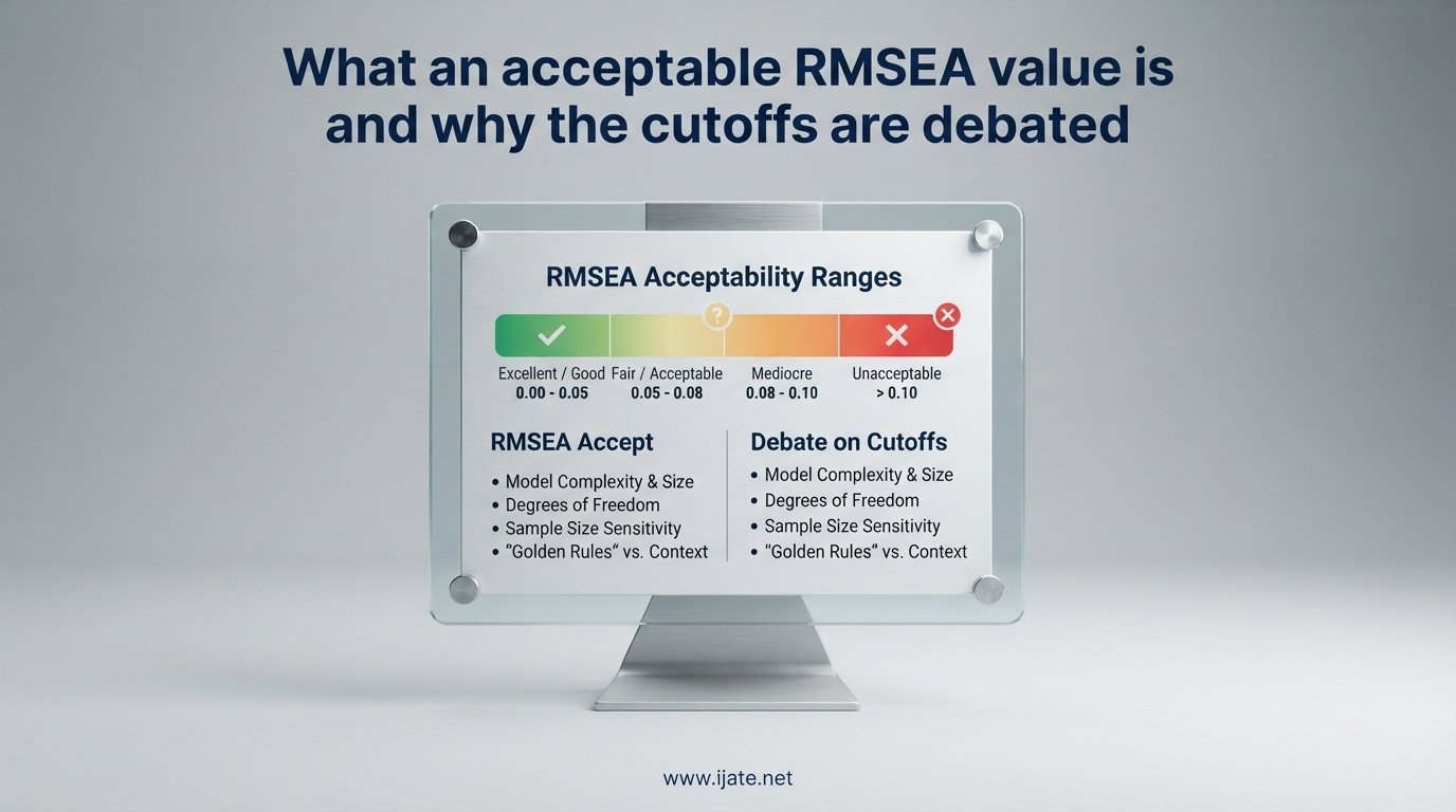
According to Browne and Cudeck (1993), an RMSEA value of 0.05 or lower indicates a close fit, meaning your model approximates the data well. Values between 0.05 and 0.08 indicate a reasonable error of approximation, which is acceptable in most applied research. Values between 0.08 and 0.10 suggest a mediocre fit, and anything above 0.10 is considered poor and usually grounds for rejecting the model.

Then Hu and Bentler (1999) entered the conversation and complicated things. Their widely cited simulation study recommended a stricter cutoff of 0.06 for RMSEA when combined with other indices like SRMR below 0.08. This recommendation came from Monte Carlo simulations that tested how well various cutoffs detected misspecified models while avoiding false rejections of correctly specified ones.

Here is the breakdown most researchers use today:

RMSEA below 0.05: Close fit, generally considered excellent.
RMSEA 0.05 to 0.08: Reasonable fit, acceptable for most publications.
RMSEA 0.08 to 0.10: Mediocre fit, requires justification.
RMSEA above 0.10: Poor fit, model needs revision.

The 0.05 threshold became a kind of golden rule because it was easy to remember and easy to enforce. Reviewers started treating it as a pass-fail line, and graduate students internalized it as the target they had to hit. But that rigid application was never what Browne and Cudeck intended. They described these as guidelines, not commandments, and they explicitly warned against using them without considering sample size and model complexity.

Why RMSEA Cutoffs Are Debated

Here is where things get contentious. The debate over RMSEA cutoffs is not a minor academic squabble. It strikes at the core of how researchers evaluate model fit, and it has real consequences for what gets published and what gets rejected.

The first problem is that cutoffs were derived from simulations, and simulations depend on assumptions that may not match your data. Chen, Curran, Bollen, Kirby, and Paxton (2008) ran extensive Monte Carlo studies published in PMC and found that fixed cutoff points perform poorly across different conditions. A 0.05 cutoff rejected too many valid models when sample sizes were small, and it failed to catch genuinely misspecified models in other conditions.

The second problem is that cutoffs ignore context. An RMSEA of 0.07 in a confirmatory factor analysis with 800 participants and 12 indicators means something very different from the same value in a path model with 80 participants and 3 observed variables. Treating both as equally acceptable or equally problematic makes no statistical sense.

The third problem, and perhaps the most overlooked, is the low degrees of freedom issue. Kenny, Kaniskan, and McCoach (2015) demonstrated that RMSEA is fundamentally broken for models with few degrees of freedom. When df is 1 or 2, RMSEA tends to be inflated even for correctly specified models. They found that a perfectly good model with df equal to 1 could produce an RMSEA above 0.10, which would trigger automatic rejection under standard cutoff rules.

As one Reddit user on r/AskStatistics put it, the problem with cutoff guidelines is that they are just guidelines. An RMSEA of 0.089 is not magically better than 0.090. Yet journal reviewers routinely reject models at 0.091 while accepting models at 0.089, treating an arbitrary line as though it were a law of nature.

The broader critique is that fit indices, including RMSEA, should supplement judgment rather than replace it. No single number can tell you whether your model is theoretically sound, whether your indicators measure what you claim they measure, or whether your specification decisions make sense. Cutoffs give a false sense of objectivity to what is ultimately a judgment call.

How Sample Size Distorts RMSEA

Sample size is the single biggest confound in RMSEA interpretation, and it causes more confusion among researchers than any other factor. Understanding this distortion is essential before you panic over a high value.

With small samples, RMSEA tends to be inflated. The formula divides by sample size minus one, and when N is small, random sampling error inflates the chi-square statistic disproportionately. This means a correctly specified model tested with 100 participants might show an RMSEA of 0.09, while the exact same model tested with 1,000 participants might show 0.04. The model did not change. The sample did.

With large samples, the opposite problem emerges for the chi-square test. Chi-square is extremely sensitive to sample size, so with N above 500, even trivially misspecified models get rejected. Researchers turned to RMSEA precisely because it is less sensitive to sample size than chi-square. But less sensitive does not mean immune.

Chen and colleagues showed in their 2008 simulation that rejection rates for properly specified models varied dramatically by sample size. At N equal to 100, the 0.05 cutoff rejected nearly 30 percent of correctly specified models. At N equal to 1,000, the same cutoff rejected far fewer. This means applying a fixed cutoff across studies with different sample sizes is statistically indefensible.

The practical takeaway is that you must report your sample size alongside your RMSEA and interpret the value in that context. A value of 0.08 with N equal to 85 deserves more leniency than the same value with N equal to 850. Reviewers who understand SEM will recognize this, and those who do not can often be educated with a brief explanation.

Reading the 90% Confidence Interval and PCLOSE

The RMSEA point estimate alone tells only part of the story. The 90% confidence interval around that estimate is equally important, and many methodologists argue it matters more than the point value itself.

David Kenny, whose website on SEM fit is cited by Google’s AI Overview, recommends looking at whether the lower bound of the 90% confidence interval includes or approaches zero. If the lower bound is near zero, your model is consistent with close fit even if the point estimate looks borderline. If both bounds exceed 0.08, your model genuinely struggles.

For example, an RMSEA point estimate of 0.06 with a 90% CI of 0.000 to 0.092 tells a different story than 0.06 with a CI of 0.041 to 0.079. The first suggests your model might fit closely. The second says your model fits reasonably but is unlikely to fit closely. Same point estimate, completely different conclusion.

PCLOSE is the p-value associated with the null hypothesis that the population RMSEA equals 0.05, meaning close fit. A PCLOSE above 0.05 means you cannot reject the close-fit hypothesis, which is good news. A PCLOSE below 0.05 means your model is significantly worse than close fit.

PCLOSE has its own critics. Some methodologists argue it suffers from the same sample size sensitivity as the overall chi-square test. With very large samples, PCLOSE can flag models that are practically fine. With small samples, it can fail to detect genuine problems. Treat it as supplementary information rather than a definitive verdict.

The best practice is to report all three pieces: the point estimate, the full confidence interval, and PCLOSE. Together they paint a more complete picture than any single number. A reviewer who sees all three is more likely to engage thoughtfully with your model fit than one who sees only a point estimate above a magic line.

RMSEA vs Other Fit Indices: CFI, TLI, and SRMR

No single fit index tells the whole story, which is why methodologists recommend reporting multiple indices and evaluating them together. RMSEA is one voice in a chorus, and sometimes the voices disagree.

Here is how the major SEM fit indices compare, including their standard cutoffs and what they measure:

RMSEA measures absolute approximate fit with a penalty for complexity. Standard cutoff: below 0.06 (Hu and Bentler) or below 0.08 (Browne and Cudeck). Lower is better.

CFI, the Comparative Fit Index, measures improvement over the null model with a penalty for complexity. Standard cutoff: above 0.95 (Hu and Bentler) or above 0.90 (older convention). Higher is better.

TLI, the Tucker-Lewis Index, also measures improvement over the null model but with a steeper complexity penalty than CFI. Standard cutoff: above 0.95 (Hu and Bentler). Higher is better.

SRMR, the Standardized Root Mean Square Residual, measures the average standardized residual between observed and model-implied covariance matrices. Standard cutoff: below 0.08 (Hu and Bentler). Lower is better.

When these indices conflict, researchers face a genuine dilemma. A common scenario from statistics forums: CFI is 0.96, TLI is 0.94, SRMR is 0.04, but RMSEA is 0.09. Three indices say the model is fine, but RMSEA flags a problem. This often happens with small degrees of freedom or moderate sample sizes.

Hu and Bentler (1999) proposed a dual-cutoff strategy for exactly this situation. Rather than relying on any single index, they recommended evaluating at least one absolute index like RMSEA or SRMR alongside one incremental index like CFI or TLI. If both types meet their cutoffs, you can be more confident in your model. If they disagree, investigate model specification before concluding your model is wrong.

One forum insight worth noting: users report that perfect fit indices, where CFI equals 1.00 and RMSEA equals 0.000, often raise red flags about overfitting or underidentification. Models that fit too perfectly are suspicious. A little misfit is more believable than no misfit.

What to Do When Your RMSEA Is Borderline

Borderline RMSEA values between 0.08 and 0.10 cause more anxiety than any other scenario in SEM. You have a model that theoretically makes sense, your other indices look acceptable, but RMSEA sits in the mediocre range. Here is a practical approach.

First, check your degrees of freedom. If df is below 5, Kenny and colleagues demonstrated that RMSEA is likely inflated regardless of model quality. In their 2015 paper, they recommended reporting RMSEA with caution for low-df models and suggested that researchers consider not reporting RMSEA at all when df equals 1. Some journals now accept this argument.

Second, examine the confidence interval. If the lower bound of the 90% CI includes zero or is very near zero, your model is statistically consistent with close fit. Report the full interval and argue that the point estimate is imprecise rather than damning.

Third, look at modification indices. If a few large modification indices suggest adding one or two theoretically justified parameters, doing so may substantially improve RMSEA. But never add parameters solely to chase a cutoff. Each modification must have a theoretical rationale.

Fourth, consider whether your model type inherently produces higher RMSEA. Confirmatory factor analysis models with few indicators per factor, longitudinal models with correlated residuals, and models with categorical data all tend to produce inflated RMSEA. Context matters.

Fifth, prepare to defend your choices to reviewers. Many reviewers expect RMSEA below 0.08 without understanding the debate. Cite Chen (2008) on sample size effects, cite Kenny (2015) on low degrees of freedom, and explain that the Browne and Cudeck guidelines were never meant as rigid thresholds. A well-referenced defense often works better than a silent acceptance of rejection.

Finally, remember that fit indices supplement but never replace theoretical judgment. A model with RMSEA of 0.07 that makes theoretical sense is more valuable than a model with RMSEA of 0.03 built by chasing modification indices. Good science weighs both statistical and substantive evidence.

FAQs

Conclusion

Understanding what an acceptable RMSEA value is requires more than memorizing cutoff numbers. The 0.05 threshold from Browne and Cudeck (1993) and the 0.06 recommendation from Hu and Bentler (1999) are useful starting points, but they were never designed as universal pass-fail lines.

Sample size, degrees of freedom, model complexity, and confidence intervals all shape what your RMSEA value means in practice. A value that looks poor on paper may be entirely defensible given your data and model structure, while a value that looks excellent may hide overfitting or specification problems.

The best approach is to report RMSEA alongside its confidence interval and PCLOSE, pair it with at least one incremental index like CFI or TLI, and interpret all fit indices in the context of your sample size and degrees of freedom. When reviewers challenge a borderline value, you now have the citations and reasoning to defend your model intelligently. That is what understanding an acceptable RMSEA value and why the cutoffs are debated really comes down to.

Key References

Browne, M. W., & Cudeck, R. (1993). Alternative ways of assessing model fit. In K. A. Bollen & J. S. Long (Eds.), Testing Structural Equation Models (pp. 136-162). Sage.

Hu, L., & Bentler, P. M. (1999). Cutoff criteria for fit indexes in covariance structure analysis: Conventional criteria versus new alternatives. Structural Equation Modeling, 6(1), 1-55.

Chen, F., Curran, P. J., Bollen, K. A., Kirby, J., & Paxton, P. (2008). An empirical evaluation of the use of fixed cutoff points in RMSEA test statistic in structural equation models. Sociological Methods & Research, 36(4), 462-494.

Kenny, D. A., Kaniskan, B., & McCoach, D. B. (2015). The performance of RMSEA in models with small degrees of freedom. Sociological Methods & Research, 44(3), 486-507.

Kenny, D. A. (2024). SEM: Measuring Model Fit. Retrieved from davidakenny.net.