What Sphericity Is and How to Handle a Violation (2026 Guide)?

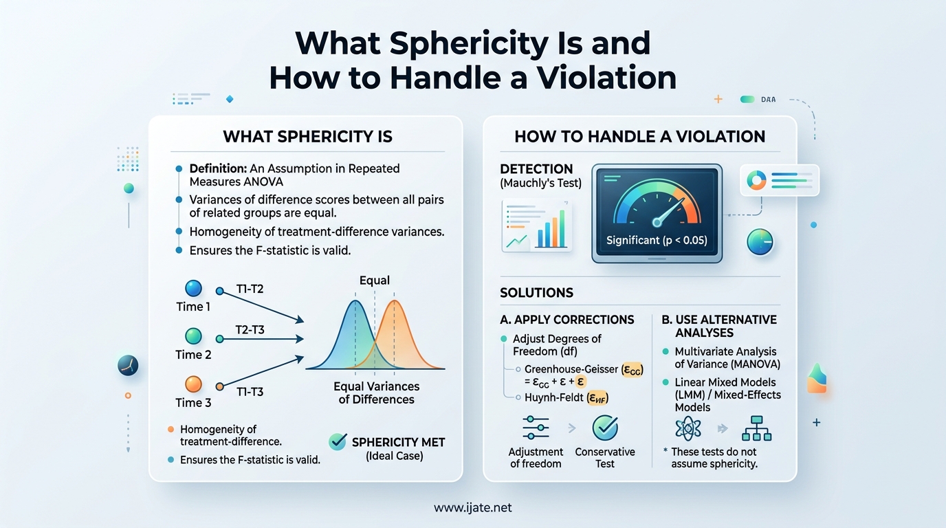
Sphericity is the assumption that the variances of the differences between all possible pairs of related groups (levels of a within-subject factor) are equal. It is a core requirement of repeated measures ANOVA. When sphericity is violated, the standard F-test becomes too liberal, inflating your Type I error rate and producing false positives at a higher rate than your chosen alpha level.

If you run repeated measures designs with three or more conditions, you need to understand sphericity, know how to test for it, and know exactly what to do when it fails. This guide walks through the definition, testing procedure (Mauchly’s test), epsilon interpretation, the two main correction methods (Greenhouse-Geisser and Huynh-Feldt), practical examples with real numbers, software-specific guidance, and APA reporting standards.

Our team has spent years analyzing repeated measures data across psychology, education, and biomedical research. We have seen every sphericity scenario imaginable, from clean datasets that pass Mauchly’s test effortlessly to severely violated assumptions that require switching to MANOVA. This guide distills what researchers actually need to know, in plain language, with decision rules you can apply immediately.

What Sphericity Means in Statistics

Sphericity (sometimes called circularity) is the condition where the variances of the differences between all combinations of related groups are equal. In a repeated measures design with three or more conditions, you can calculate difference scores for every pair of conditions. Sphericity requires that the variance of those difference scores is the same across all pairs.

Think of it this way: if you have conditions A, B, and C, you can form three difference-score variables (A minus B, A minus C, and B minus C). Sphericity says the variance of each of those difference-score variables should be the same. When they are, the standard ANOVA F-test is valid. When they are not, the F-test is positively biased.

Sphericity vs. Compound Symmetry

People often confuse sphericity with compound symmetry, but they are not identical. Compound symmetry is a stricter condition that requires two things: all variances are equal, and all covariances are equal. Sphericity is less demanding. It requires only that the variances of the differences are equal, which is a subset of what compound symmetry demands.

In practical terms, if your data meets compound symmetry, it automatically meets sphericity. But data can meet sphericity without meeting compound symmetry. This distinction matters because some textbooks and software packages reference compound symmetry as a shorthand, which can create confusion when Mauchly’s test gives one answer and compound symmetry checks give another.

Why Sphericity Matters for Repeated Measures ANOVA

The standard univariate repeated measures ANOVA F-test assumes sphericity. The F-statistic is calculated using degrees of freedom that are only correct when sphericity holds. When the assumption is met, the F-statistic follows the expected F-distribution under the null hypothesis, and your p-values are accurate.

When sphericity is violated, the actual Type I error rate exceeds the nominal alpha level you set. If you think you are testing at p < .05, you might actually be testing at p < .10 or worse. This means you will reject the null hypothesis too often, finding “significant” effects that are really just noise.

The severity of the inflation depends on how badly sphericity is violated. A mild violation produces a small increase in false positives. A severe violation can nearly double your Type I error rate. This is why sphericity is not a minor technical detail to glance at and dismiss. It directly affects the validity of your conclusions.

Consequences of a Sphericity Violation

The main consequence of violating sphericity is an inflated F-statistic. The F-ratio becomes larger than it should be because the error term is underestimated. A larger F means a smaller p-value, which means you are more likely to declare a result significant when it is not.

Box showed decades ago that the degree of Type I error inflation depends on the degree of sphericity violation, measured by epsilon. When epsilon drops below 0.75, the inflation becomes substantial. When epsilon approaches its lower bound of 1/(k-1) where k is the number of levels, the F-test can become badly misleading without correction.

Researchers on forums like r/statistics and Stack Exchange frequently report confusion when their repeated measures ANOVA shows significance but a mixed model does not. Often, the explanation is that sphericity was violated and the ANOVA result was a false positive. Checking sphericity before trusting your F-test prevents this scenario.

How to Test for Sphericity: Mauchly’s Test

Mauchly’s test of sphericity is the standard statistical test used to evaluate whether the sphericity assumption holds. Developed by John Mauchly in 1940, it produces a test statistic called Mauchly’s W and an associated p-value. The null hypothesis is that sphericity holds, meaning the variances of all pairwise differences are equal.

Here is the critical interpretation rule: if Mauchly’s test is not significant (p > .05), you fail to reject the null hypothesis, and you can assume sphericity holds. You report the standard “sphericity assumed” F-test results. If Mauchly’s test is significant (p < .05), sphericity is violated, and you must apply a correction or switch to an alternative method.

Interpreting Mauchly’s W and p-value

Mauchly’s W ranges from 0 to 1. A W value close to 1 indicates that the data closely matches the sphericity assumption. Lower W values indicate greater departure from sphericity. The associated p-value tells you whether that departure is statistically significant.

SPSS, R, and Python all report Mauchly’s W alongside the approximate chi-square statistic, degrees of freedom, and p-value (labeled as “Sig.” in SPSS). You need only check the p-value to make your decision. The W and chi-square values are useful for reporting but not strictly necessary for interpretation.

When Mauchly’s Test Is Unnecessary

Mauchly’s test is only relevant when your within-subject factor has three or more levels. With only two levels, there is only one pairwise difference, so the concept of equal variances of differences is moot. Sphericity cannot be violated with a two-level factor because there is nothing to compare.

Many researchers misunderstand this. They panic when SPSS does not produce a Mauchly’s test row for a two-condition design, thinking something went wrong. Nothing went wrong. The software simply recognizes that the test is undefined for two levels.

For between-subject factors, sphericity does not apply at all. Sphericity is exclusively a within-subject (repeated measures) concept. Forum posts regularly ask whether sphericity matters for between-subjects ANOVA, and the answer is always no.

Limitations of Mauchly’s Test

Mauchly’s test has well-documented weaknesses that every researcher should know. With small sample sizes, the test lacks statistical power and often fails to detect real violations. You might get a non-significant result simply because you did not have enough participants, not because sphericity truly holds.

With large sample sizes, the opposite problem occurs. Mauchly’s test becomes overly sensitive and flags tiny, practically meaningless deviations as significant violations. A dataset with 500 participants might produce a significant Mauchly’s test even when the actual violation is negligible and epsilon is close to 1.

Because of these limitations, some statisticians recommend always applying a correction regardless of Mauchly’s test result. Maxwell and Delaney, in their widely cited textbook, argue that the Greenhouse-Geisser correction is conservative enough to use universally without meaningful loss of power. This is a defensible position, especially for researchers who want a simple, consistent workflow.

Understanding Epsilon in Sphericity Testing

Epsilon (written as the Greek letter epsilon) is a descriptive statistic that quantifies how badly sphericity is violated. It ranges from a lower bound of 1/(k-1), where k is the number of levels of the within-subject factor, up to a maximum of 1.0. An epsilon of 1.0 means sphericity is perfectly met. Lower values indicate more severe violations.

For a design with 4 conditions, the lower bound for epsilon is 1/(4-1) = 0.333. For 5 conditions, it is 1/(5-1) = 0.25. The more levels you have, the lower the possible floor for epsilon, and the more room there is for sphericity to be badly violated.

What Epsilon Measures

Epsilon directly relates to the degree of Type I error inflation you can expect. When epsilon equals 1.0, there is no inflation. When epsilon drops, the inflation increases. An epsilon of 0.5 means your actual Type I error rate could be roughly double your nominal alpha.

The correction methods work by multiplying the degrees of freedom by epsilon. If your original degrees of freedom for the effect are 3 and the error df is 60, and epsilon is 0.6, the corrected df become 3 times 0.6 = 1.8 and 60 times 0.6 = 36. The F-statistic itself does not change, but the critical value used to evaluate it does, because the F-distribution changes shape with different degrees of freedom.

This is why corrections make it harder to reach significance. They reduce the degrees of freedom, which adjusts the F-distribution to account for the sphericity violation. The p-value increases, protecting you from false positives.

Three Epsilon Estimates

There are three commonly reported epsilon estimates, each calculated differently:

Greenhouse-Geisser epsilon: This is the most conservative estimate. It tends to underestimate the true degree of sphericity, meaning it slightly overcorrects. It is the most widely used and the safest default choice.

Huynh-Feldt epsilon: This is a less conservative estimate. It tends to be slightly higher than Greenhouse-Geisser, meaning it corrects less aggressively. It was designed to address the tendency of Greenhouse-Geisser to overcorrect, especially when epsilon is near or above 0.75.

Lower-bound epsilon: This is the most conservative possible value: 1/(k-1). It assumes the worst-case scenario for sphericity. It almost always overcorrects, making it unnecessarily strict. Most methodologists recommend against using it unless you have no other option, because it dramatically reduces statistical power.

Greenhouse-Geisser Correction

The Greenhouse-Geisser correction is the most widely used method for handling sphericity violations. It was developed by Samuel Greenhouse and Seymour Geisser in 1959. The correction adjusts the degrees of freedom of the F-test by multiplying them by the Greenhouse-Geisser epsilon estimate.

For example, if you have a within-subject factor with 4 levels (original effect df = 3, error df = 57) and your Greenhouse-Geisser epsilon is 0.55, the corrected degrees of freedom become 3 times 0.55 = 1.65 and 57 times 0.55 = 31.35. SPSS, R, and Python all report these adjusted df alongside the corrected p-value.

The correction is straightforward to apply because the software does it automatically. Your job is to know when to read the corrected row instead of the “sphericity assumed” row in your output.

When to Use the Greenhouse-Geisser Correction

The standard guideline, based on recommendations from Girden (1992) and widely adopted in statistical software documentation, is to use the Greenhouse-Geisser correction when epsilon is less than 0.75. Below this threshold, the Greenhouse-Geisser estimate is considered more reliable because the Huynh-Feldt estimate can be too liberal.

The Greenhouse-Geisser correction is deliberately conservative. It tends to slightly overcorrect, meaning it may reduce your power somewhat. This is a feature, not a bug. A small loss of power is a reasonable price for protecting against inflated Type I error rates. Finding a non-significant result with Greenhouse-Geisser when the uncorrected test was significant is a common and expected outcome.

Many experienced researchers use Greenhouse-Geisser as their default correction regardless of the epsilon value. This simplifies the workflow and avoids the complexity of deciding between corrections. The slight conservatism is acceptable in most research contexts.

Huynh-Feldt Correction

The Huynh-Feldt correction was developed by Huynh and Feldt in 1976 as an improvement on the Greenhouse-Geisser method. The Greenhouse-Geisser epsilon has a known tendency to underestimate the true population epsilon, especially when the true value is close to 1. The Huynh-Feldt estimate corrects for this bias.

The result is that Huynh-Feldt epsilon is almost always higher than Greenhouse-Geisser epsilon for the same dataset. A higher epsilon means less correction, which means more degrees of freedom retained and more statistical power preserved.

When to Use the Huynh-Feldt Correction

Following Girden’s recommendation, the Huynh-Feldt correction is preferred when epsilon is greater than 0.75. At this level, the sphericity violation is relatively mild, and the more conservative Greenhouse-Geisser correction would overcorrect unnecessarily. The Huynh-Feldt correction provides a better balance between Type I error protection and statistical power.

However, the Huynh-Feldt correction can sometimes produce epsilon values greater than 1.0. When this happens, the standard practice is to set epsilon to 1.0, which means no correction is applied. This is equivalent to reporting the “sphericity assumed” results.

Researchers on statistics forums frequently ask about the Huynh-Feldt vs Greenhouse-Geisser choice. The decision rule based on the 0.75 threshold is the most widely cited and is supported by simulation studies showing it provides good Type I error control across a range of scenarios.

Which Correction Should You Use

The decision between Greenhouse-Geisser and Huynh-Feldt comes down to a single threshold: 0.75. Here is the straightforward decision rule that works for the vast majority of research situations.

If Greenhouse-Geisser epsilon is less than 0.75: Use the Greenhouse-Geisser correction. The violation is severe enough that the conservative estimate is warranted. Huynh-Feldt would be too liberal at this level.

If Greenhouse-Geisser epsilon is 0.75 or higher: Use the Huynh-Feldt correction. The violation is mild enough that the more powerful estimate is appropriate. Greenhouse-Geisser would overcorrect and waste statistical power.

If you want a simple rule that always works: Always use Greenhouse-Geisser. It is never badly wrong. It may be slightly conservative when epsilon is high, but it will never produce an inflated Type I error rate. This is the approach recommended by Maxwell and Delaney.

Greenhouse-Geisser vs. Huynh-Feldt Comparison

The two corrections differ in several key ways. Greenhouse-Geisser is more conservative, meaning it is less likely to produce a significant result but also less likely to produce a false positive. Huynh-Feldt is more liberal, meaning it retains more power but carries a slightly higher risk of Type I error when the violation is severe.

In practice, the two corrections usually lead to the same conclusion. When the uncorrected p-value is well below .05 or well above .05, both corrections give the same answer. The corrections matter most when the uncorrected p-value hovers near the .05 threshold, and that is when the choice between them becomes important.

The Lower-Bound Estimate and Why to Avoid It

The lower-bound estimate is the most conservative possible correction. It sets epsilon to 1/(k-1), which is the minimum possible value. For a 4-level factor, that is 0.333. For a 5-level factor, it is 0.25. This correction drastically reduces the degrees of freedom and dramatically cuts statistical power.

The lower-bound estimate assumes the absolute worst-case scenario for sphericity. In reality, violations are rarely that extreme. Using this correction is like wearing a winter coat in mild weather. It protects you, but it is overkill.

Most software reports the lower-bound estimate alongside Greenhouse-Geisser and Huynh-Feldt. We recommend ignoring it unless you have a specific theoretical reason to expect the worst possible violation pattern. Both Greenhouse-Geisser and Huynh-Feldt provide better corrections that are grounded in your actual data rather than a hypothetical extreme.

Forum discussions reveal that undergraduate students often default to the lower-bound correction because it seems “safest.” This is a mistake. The unnecessary power loss can cause you to miss real effects. Use Greenhouse-Geisser or Huynh-Feldt instead.

Step-by-Step Example with Variance Calculations

To make sphericity concrete, let us walk through a numerical example. Suppose you have a repeated measures design with 10 participants measured across three conditions: Baseline, Treatment, and Follow-up. You want to test whether the three conditions differ significantly.

First, calculate the difference scores for each participant. You need three sets of differences: Baseline minus Treatment, Baseline minus Follow-up, and Treatment minus Follow-up. Each participant gets three difference scores.

Next, calculate the variance of each set of difference scores. Suppose the variance of Baseline minus Treatment is 4.2, the variance of Baseline minus Follow-up is 4.5, and the variance of Treatment minus Follow-up is 12.1. These are clearly not equal. The third pair has a much larger variance than the first two.

This means sphericity is violated. The differences between Treatment and Follow-up are much more variable than the differences involving Baseline. Perhaps the Treatment effect is unstable across participants, with some showing large changes and others showing small ones. Mauchly’s test would likely confirm this with a significant p-value.

When sphericity is this clearly violated, you would apply the Greenhouse-Geisser correction (assuming epsilon is below 0.75, which it almost certainly would be given the variance disparity). The corrected F-test would give you an honest p-value that accounts for the unequal variances.

If the variance of all three difference-score sets had been similar, say 4.2, 4.5, and 4.3, sphericity would be essentially met. Mauchly’s test would likely return a non-significant result, and you could use the standard “sphericity assumed” F-test.

Alternatives When Sphericity Is Severely Violated

When epsilon is very low (below 0.50 or so), even corrected F-tests may be unreliable. In these cases, you have two strong alternatives that do not assume sphericity at all.

MANOVA as an Alternative

The multivariate approach to repeated measures ANOVA does not assume sphericity. Instead of treating the repeated measures as a single within-subject factor, MANOVA treats the difference scores (or the repeated measures themselves) as multiple dependent variables in a multivariate analysis.

MANOVA uses test statistics like Wilks’ lambda, Pillai’s trace, Hotelling’s trace, and Roy’s largest root. None of these require sphericity. When sphericity is severely violated, MANOVA can actually be more powerful than the corrected univariate F-test.

The trade-off is that MANOVA requires a larger sample size to be reliable. A common rule of thumb is that you need more cases than the number of dependent variables. With small samples, MANOVA can be underpowered, and the corrected univariate test may be preferable despite the sphericity violation.

Mixed-Effects Models

Linear mixed-effects models (also called multilevel models or hierarchical linear models) handle repeated measures data without assuming sphericity. They model the covariance structure of the repeated observations directly, allowing you to specify different patterns such as autoregressive, compound symmetry, or unstructured.

Mixed models are increasingly recommended as the modern alternative to repeated measures ANOVA. They handle missing data more gracefully, accommodate unequal group sizes, and let you model time as a continuous variable. Most modern statistics packages support them.

The downside is increased complexity. Specifying and interpreting mixed models requires more statistical knowledge than running a standard ANOVA. For simple designs where sphericity corrections are adequate, the extra complexity may not be justified.

Software Implementation Notes

Different software packages handle sphericity testing and corrections in different ways. Here is what you need to know for the three most common tools.

SPSS: Reading Mauchly’s Test Output

SPSS provides Mauchly’s test automatically when you run a repeated measures ANOVA through the General Linear Model menu. The output includes a table titled “Mauchly’s Test of Sphericity” with columns for Mauchly’s W, approximate chi-square, degrees of freedom, and significance (the p-value).

If the significance value is greater than .05, look at the “Sphericity Assumed” row in the “Tests of Within-Subjects Effects” table. If it is .05 or less, use either the “Greenhouse-Geisser” or “Huynh-Feldt” row based on the epsilon value reported in the Mauchly’s test table. SPSS conveniently lists all three correction rows alongside the sphericity-assumed row, so you just need to pick the right one.

SPSS also reports the lower-bound correction row. As discussed, ignore this unless you have a specific reason to use it.

R: Using ezANOVA or afex

In R, the most user-friendly way to run a repeated measures ANOVA with sphericity testing is through the ez package (ezANOVA function) or the afex package (aov_ez function). Both automatically report Mauchly’s test and the Greenhouse-Geisser and Huynh-Feldt corrections.

With ezANOVA, the output includes a Mauchly’s test result and a note telling you which correction to use. The afex package gives you the corrected ANOVA table directly and lets you specify the correction method using the correction argument. Set correction = “GG” for Greenhouse-Geisser or correction = “HF” for Huynh-Feldt.

For mixed models, the lme4 package with lmer() is the standard choice. The emmeans package can then compute estimated marginal means and pairwise comparisons.

Python: Pingouin and Statsmodels

In Python, the pingouin library provides the easiest path to sphericity testing. The pg.rm_anova() function runs a repeated measures ANOVA and automatically reports Mauchly’s test, Greenhouse-Geisser epsilon, and Huynh-Feldt epsilon. Set the correction parameter to True to get corrected p-values.

Pingouin also has a dedicated pg.sphericity() function that tests for sphericity on its own, useful for exploratory checks before running the full ANOVA.

Statsmodels offers repeated measures capabilities through its ANOVA and mixed-effects model functions, but the sphericity testing is less automated. For sphericity-specific work, pingouin is the better starting point.

How to Report Sphericity Results in APA Format

Reporting sphericity results in APA format requires mentioning Mauchly’s test, the outcome, and which correction you used (if any). Here is the standard pattern.

When sphericity is not violated: Report that Mauchly’s test was non-significant and you used the uncorrected results. Example: “Mauchly’s test indicated that the assumption of sphericity had not been violated, chi-square(2) = 2.34, p = .31.”

When sphericity is violated: Report the significant Mauchly’s test result and identify which correction you applied. Example: “Mauchly’s test indicated that the assumption of sphericity had been violated, chi-square(5) = 18.76, p = .002. Therefore, degrees of freedom were corrected using Greenhouse-Geisser estimates of sphericity (epsilon = 0.62).”

Reporting the corrected ANOVA result: Include the corrected degrees of freedom (which will be non-integer values) along with the F-statistic and p-value. Example: “The effect of condition was significant, F(1.86, 34.12) = 7.45, p = .002, partial eta squared = 0.29.”

Always report the corrected degrees of freedom with two decimal places, as recommended by APA style. Report epsilon to two decimal places as well. Include the effect size (partial eta squared or generalized eta squared) alongside the F-test for completeness.

Forum users frequently ask how to report sphericity in a thesis or published paper. The key is transparency: always state what Mauchly’s test showed, what correction you used, and why. Reviewers and advisors want to see that you understood the assumption and handled it correctly.

FAQs

Conclusion: Your Sphericity Checklist

Understanding what sphericity is and how to handle a violation comes down to a few key steps. First, recognize that sphericity only matters for within-subject factors with three or more levels. Second, check Mauchly’s test in your software output. Third, if the test is significant, apply Greenhouse-Geisser when epsilon is below 0.75 or Huynh-Feldt when it is 0.75 or above. Fourth, report the corrected results with adjusted degrees of freedom in APA format.

If epsilon is extremely low, consider MANOVA or a mixed-effects model as alternatives that do not require the sphericity assumption at all. And remember that Mauchly’s test has limitations with very small or very large samples, so some researchers prefer to always apply the Greenhouse-Geisser correction as a safeguard.

We recommend bookmarking this page or saving the decision rule for quick reference. Sphericity is one of those statistical concepts that becomes easy once you have run through it a few times. The decision tree is simple, the corrections are automatic in modern software, and the APA reporting follows a predictable pattern. Once you internalize these steps, handling sphericity violations becomes second nature.