Standard Error of Measurement for Individual Test Scores 2026 Guide

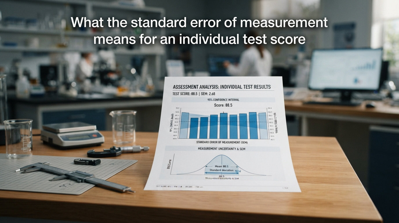
Every test score you have ever received is wrong. Not wildly wrong, and not because of a grading mistake, but wrong in a quiet, measurable way. The number printed on a score report is an estimate of something deeper that psychologists and educators call a true score, and the gap between the two is captured by one of the most misunderstood statistics in all of testing: the standard error of measurement. When we talk about what the standard error of measurement individual test score interpretation really means, we are asking how much wiggle room surrounds a single result and whether that wiggle room changes the decisions we make about a person.

If you are an educator reading a student’s assessment results, a clinician interpreting a cognitive battery, a test developer building a new instrument, or a student of psychometrics trying to pass a statistics exam, understanding SEM changes how you read every score report that lands on your desk. This article breaks down what SEM is, how to calculate it, how to build a confidence interval around an individual score, and why ignoring it can lead to bad decisions about real people.

What Is the Standard Error of Measurement?

The standard error of measurement, almost always abbreviated as SEM, is the standard deviation of the errors that surround an individual’s observed test score. In simpler terms, it tells you how much a single person’s score would bounce around if they took the same test over and over again without learning anything in between. A smaller bounce means a more precise test. A larger bounce means the observed number on the page could be quite far from the person’s actual ability level.

To understand SEM, you need three foundational concepts from classical test theory. The first is the true score, which is the hypothetical, perfectly accurate reflection of whatever the test is measuring. The second is the observed score, which is the number the test taker actually receives. The third is measurement error, the random difference between the two. Classical test theory treats every observed score as the sum of the true score plus random error, and SEM is the yardstick for that error.

Think of SEM as the testing world’s version of a margin of error in political polling. When a poll says a candidate has 52 percent support plus or minus 3 points, nobody treats the 52 as gospel. The same logic applies to a test score. If a student scores 105 on a reading test with a SEM of 5, the score is not really 105. It is somewhere in a band around 105, and SEM defines the width of that band.

This is why SEM matters so much for an individual test score specifically. Group-level statistics smooth out random error across hundreds of test takers. But when you are looking at one person’s result, that random error is at full strength and SEM is the only tool you have to quantify it.

The SEM Formula Explained

The most common formula for the standard error of measurement in classical test theory is straightforward once you break it into pieces. SEM equals the standard deviation of the test scores multiplied by the square root of one minus the reliability coefficient. Written out, it looks like this: SEM = SD multiplied by the square root of (1 minus r).

Each piece of the formula carries meaning. SD, the standard deviation, measures how spread out all the test scores are across the population that took the test. The reliability coefficient, usually symbolized by a lowercase r, measures how consistent the test is, typically ranging from 0 to 1. Subtracting r from 1 tells you the proportion of score variance that comes from error rather than true differences in ability. Taking the square root converts that proportion back into the original score units.

Here is a step-by-step SEM calculation you can follow with your own data.

Step 1: Find the standard deviation of the test. Suppose a standardized math test has a population SD of 15 scaled-score points.

Step 2: Locate the test’s reliability coefficient from the technical manual. Say the internal consistency reliability is reported as 0.91.

Step 3: Subtract the reliability from 1. That gives you 1 minus 0.91, which equals 0.09.

Step 4: Take the square root of that result. The square root of 0.09 is 0.30.

Step 5: Multiply by the standard deviation. Fifteen multiplied by 0.30 equals 4.5.

The SEM for this test is 4.5 scaled-score points. That single number now travels with every individual score report and tells you the typical size of measurement error for any one test taker on this instrument.

Notice what the formula reveals about the relationship between reliability and SEM. As reliability approaches a perfect 1.0, the term under the square root approaches zero, and SEM shrinks toward zero as well. A perfectly reliable test would have no measurement error at all. As reliability drops, SEM grows, meaning each observed score becomes a fuzzier estimate of the true score. This is why test developers fight so hard to push reliability coefficients as high as possible.

Confidence Intervals: Putting SEM to Work for Individual Scores

Knowing that a test has a SEM of 4.5 is only useful if you can turn it into a statement about a real score. That is exactly what a confidence interval does. A confidence interval takes the observed score and wraps a band around it, using the SEM as the unit of width, so you can say with a chosen level of confidence where the person’s true score probably lies.

Psychometricians typically work with two confidence levels. A 68 percent confidence interval uses plus or minus one SEM. A 95 percent confidence interval uses plus or minus roughly two SEMs, technically 1.96 SEMs for a normal distribution. These percentages come directly from the properties of the normal curve, where about 68 percent of values fall within one standard deviation of the mean and about 95 percent fall within two.

Here is how to construct a confidence interval step by step.

Step 1: Start with the individual’s observed score. Let us say a student scored 102 on the math test from our earlier example.

Step 2: Retrieve the SEM you calculated, which was 4.5 points.

Step 3: For a 68 percent confidence interval, add and subtract one SEM. The lower bound is 102 minus 4.5, equaling 97.5. The upper bound is 102 plus 4.5, equaling 106.5.

Step 4: For a 95 percent confidence interval, multiply the SEM by 1.96. That gives you 4.5 times 1.96, which is approximately 8.8. The lower bound is 102 minus 8.8, equaling 93.2. The upper bound is 102 plus 8.8, equaling 110.8.

Step 5: Interpret the result. We are 68 percent confident the student’s true math ability lies between 97.5 and 106.5. We are 95 percent confident it lies somewhere in the wider band from 93.2 to 110.8.

That is the practical meaning of SEM for an individual test score in a single paragraph. The observed score of 102 is not the story. The story is a range, and the width of that range is controlled entirely by the SEM.

One technical note is worth mentioning here. The classical SEM we just calculated is a single number that applies to every test taker regardless of where they scored. In item response theory, a more advanced framework, SEM actually changes depending on the person’s ability level. This is called the conditional standard error of measurement, or CSEM. A test tends to measure most precisely in the middle of the score range and less precisely at the extreme high and low ends. For most everyday score interpretation, the classical SEM is what you will see reported, but knowing that CSEM exists helps you understand why a test might be less reliable for someone scoring at the very top or very bottom.

Worked Example: Interpreting One Student’s Score

Let us walk through a complete scenario from start to finish so you can see how SEM changes a real-world decision. Imagine a school psychologist is reviewing the results of a norm-referenced language test for a seven-year-old student. The test manual reports a mean of 100, a standard deviation of 15, and a reliability coefficient of 0.89 for the child’s age group. The student received a standard score of 78.

First, calculate the SEM. The standard deviation is 15 and the reliability is 0.89. One minus 0.89 equals 0.11. The square root of 0.11 is approximately 0.332. Multiply 15 by 0.332 and you get a SEM of about 5 points.

Now build the 95 percent confidence interval around the student’s observed score of 78. Multiply the SEM of 5 by 1.96 to get 9.8, which rounds to about 10 points. The lower bound is 78 minus 10, giving 68. The upper bound is 78 plus 10, giving 88.

Here is where SEM becomes more than a math exercise. Many school districts use a standard score of 70 as a cutoff for certain services. This student’s observed score of 78 falls above that cutoff, which might suggest they do not qualify. But look at the confidence interval. The lower bound of the 95 percent band dips all the way to 68, which is below the cutoff. This means we cannot be statistically confident the student’s true score is above 70.

This is exactly the kind of situation where ignoring SEM leads to a bad decision. A score of 78 looks comfortably above 70, but the confidence band tells a more honest story. The student’s true ability could be anywhere from 68 to 88. Professionals writing evaluation reports should always present this range, not just the point estimate, especially when the score sits near a decision threshold.

The same logic applies to measuring growth over time. If a student scores 102 in the fall and 106 in the spring, did they really improve? Subtract the two scores and you get four points of growth. But if the SEM is 4.5, that growth is well within the margin of error. The difference could easily be random noise. Without SEM, educators would celebrate progress that the test cannot actually detect. With SEM, they can set a defensible threshold for real change, typically something like 1.96 times the combined SEM of both administrations.

Communicating this to parents and non-statisticians is part of the job. You do not need to say the word psychometrics or write the formula on a report. You simply say something like: this score is an estimate, and we are confident the student’s true level falls within this range. That single sentence captures everything SEM is trying to tell you.

SEM vs Standard Deviation vs Standard Error of the Mean

One of the most common sources of confusion in statistics, and one of the loudest complaints on statistics forums, is the mix-up between three different standard errors. SEM the measurement error, SEM the standard error of the mean, and the standard error of the estimate are all different concepts that happen to share similar names. Getting them wrong in a research report or clinical evaluation is a serious error.

Let us separate them clearly.

Standard deviation (SD) describes how spread out individual scores are across a group of people. It is a descriptive statistic for variability in a population. If a test has an SD of 15, that tells you most test takers score within 15 points above or below the mean of 100. SD describes the spread of people, not the error of a single measurement.

Standard error of measurement (SEM) describes how much error surrounds one individual’s observed score. It is about the precision of the test for a single person. SEM is always smaller than SD because it represents only the error portion of score variability, not the real differences between people. In our example with SD of 15 and reliability of 0.91, the SEM was 4.5, much smaller than 15.

Standard error of the mean (also confusingly abbreviated SEM) describes how precisely your sample mean estimates the population mean. It shrinks as your sample size grows, following the formula SD divided by the square root of n. This has nothing to do with individual test scores. It answers a completely different question about group averages.

Standard error of the estimate (SEE) shows up in regression and prediction. It tells you how much error to expect when you use a regression line to predict one variable from another. In testing contexts, SEE is sometimes used when predicting a criterion score from a test score.

If you take away one distinction from this section, make it this: standard deviation is about people, standard error of measurement is about a test’s precision for one person, and standard error of the mean is about your confidence in a group average. They answer three entirely different questions, and mixing them up is the fastest way to undermine the credibility of your score interpretation.

The simplest comparison is this. SD answers: how different are test takers from each other? SEM answers: how far off is this person’s observed score from their true score? Standard error of the mean answers: how accurate is my estimate of the group average? When you are interpreting an individual test score, only SEM is the right tool.

What Counts as a Good SEM?

People frequently ask what a good SEM looks like, and the honest answer is that it depends on the context of the test and the decisions being made. That said, there are practical guidelines you can use.

SEM is always interpreted relative to the test’s score scale, not in absolute terms. A SEM of 3 points on a 100-point scale is tight and precise. A SEM of 3 points on a 10-point scale is enormous and nearly useless. What matters is the ratio of SEM to the test’s standard deviation and the width of the resulting confidence interval compared to the decision thresholds you care about.

Here are some general rules of thumb that psychometricians use informally.

A SEM that produces a 95 percent confidence interval narrower than about one standard deviation of the test is generally considered acceptable for most educational and clinical uses. This typically corresponds to a reliability coefficient above 0.85 or so.

A SEM that produces a 95 percent confidence band wider than one full standard deviation is a red flag. Decisions based on scores from such a test carry substantial uncertainty, and the test may be inappropriate for high-stakes individual classification.

For licensing and certification exams where a single cut score determines pass or fail, test developers aim for the tightest SEM possible around the cut point. This is one reason item response theory and conditional SEM have become popular in that field. CSEM lets you verify that the test is sufficiently precise at the exact score where the decision hangs.

Several factors influence the size of SEM. Test length is a big one, because longer tests with more items tend to be more reliable and therefore have smaller SEM values. Item quality matters too, because well-written items that discriminate between high and low ability produce higher reliability. The heterogeneity of the test-taking population affects SD, which feeds directly into the SEM formula. And the scoring model, whether classical or item response theory, changes how SEM behaves across the score range.

Adaptive tests, which select items tailored to each test taker’s ability level, deserve a special mention. Computerized adaptive testing can achieve a smaller SEM at any given ability level compared to a fixed-form test of the same length, because it concentrates items where they provide the most information. This is why adaptive assessments like NWEA’s MAP Growth report relatively precise RIT scores with tight confidence bands even for individual students.

Why SEM Matters for High-Stakes Individual Decisions

The stakes of ignoring SEM rise dramatically when a test score triggers a consequential decision. Special education eligibility, gifted program placement, professional licensing, grade retention, and clinical diagnosis all depend on whether a score crosses a threshold. SEM determines whether that crossing is real or could be statistical noise.

Consider special education qualification, a process many school psychologists navigate daily. A common pattern is that a student scores just a few points above the eligibility cutoff, and the team must decide whether the student truly does not need services. If the SEM for that test is 5 points and the score sits 3 points above the cutoff, the confidence interval clearly encompasses scores below the cutoff. Responsible practice requires acknowledging that uncertainty in the eligibility report.

The same principle applies to passing scores on professional exams. When a standard-setting method determines the cut score, SEM defines the fuzzy zone around that cut where pass and fail decisions are genuinely ambiguous. Many testing programs now publish SEM-based bands around cut scores so that stakeholders understand the precision of the classification, and some even offer appeal or retake policies for examinees whose scores fall within the error band.

Clinical and neuropsychological assessment is another domain where SEM is indispensable. Cognitive batteries like IQ tests report confidence intervals alongside every composite score, and competent clinicians interpret the band, not just the number. A full-scale IQ of 102 with a 95 percent confidence interval of 97 to 108 paints a very different picture than a bare number on a page. It tells the clinician, the patient, and the referral source how much weight to place on the result.

Communicating SEM to non-expert audiences is part of practicing good measurement ethics. Parents, teachers, administrators, and patients deserve to know that test scores are estimates. You do not need to lecture them on classical test theory. You simply need to present the confidence band and explain in plain language that the true score probably falls within that range. This small step prevents overinterpretation, reduces disputes about borderline decisions, and builds trust in the assessment process.

Forum discussions among psychologists and educators reveal a recurring frustration that SEM is underused and frequently misunderstood. Professionals report seeing evaluation reports, published studies, and even textbooks that confuse standard error of measurement with standard error of the mean. The remedy is straightforward: always report SEM for individual scores, always present confidence intervals, and always check whether score differences exceed the error band before drawing conclusions.

FAQs

Conclusion

Understanding what the standard error of measurement means for an individual test score comes down to one idea: every score is an estimate, and SEM defines the size of the estimate’s uncertainty. The formula SEM equals SD times the square root of one minus reliability gives you a single number in the test’s own score units. Wrap that number into a 68 percent or 95 percent confidence interval and you have a defensible range for where a person’s true score actually lies.

The next time you read a score report, do not stop at the point estimate. Ask for the SEM, build the confidence band, and check whether it crosses any decision threshold that matters. That habit is the difference between treating tests as infallible oracles and treating them as the useful but imperfect tools they really are.