When to Use Repeated-Measures ANOVA? (2026 Guide)

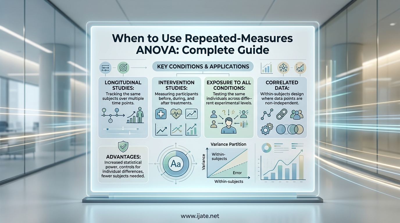
Knowing when to use repeated-measures ANOVA can make or break your statistical analysis. If you run the wrong test, you either lose statistical power or violate core assumptions that invalidate your results. In this guide, our team breaks down the exact study designs, assumptions, and decision rules that tell you whether repeated-measures ANOVA is the right choice for your data.

Repeated-measures ANOVA is a statistical test used to compare mean scores across three or more time points or conditions when the same participants are measured in each condition. It is also called a within-subjects ANOVA because the independent variable varies within each participant rather than between different groups of people.

Use repeated-measures ANOVA when your study falls into one of these two designs: (1) you are measuring changes in mean scores over three or more time points, such as a pretest, midtest, and posttest, or (2) you are comparing differences in mean scores under three or more different conditions, such as three drug dosages administered to the same patients. That is the short answer. Below, we walk through every detail you need to make the right call with confidence.

When to Use Repeated-Measures ANOVA: The Two Study Designs

The decision to use repeated-measures ANOVA comes down to one fundamental question: did the same participants provide data under multiple conditions or at multiple time points? If yes, and you have three or more levels of that within-subject factor, this test is appropriate.

There are exactly two study designs that call for repeated-measures ANOVA.

Design 1: Changes Over Three or More Time Points

The first design involves measuring the same participants at three or more distinct time points. Researchers use this design in longitudinal studies, clinical trials, and intervention studies where they want to track how a variable changes over time.

For example, imagine a clinical trial testing a new blood pressure medication. Researchers measure each patient’s systolic blood pressure at baseline (before treatment), at 6 weeks, and at 12 weeks. Because the same patients are measured three times, a repeated-measures ANOVA is the correct test to determine whether mean blood pressure differs across the three time points.

Other common examples include measuring student test scores at the start, middle, and end of a semester, or tracking employee productivity scores before, during, and after a training program. The key requirement is that every participant contributes a score at each time point.

Design 2: Differences Under Three or More Conditions

The second design involves exposing the same participants to three or more different conditions. The conditions could be different treatments, different stimuli, different dosages, or different task difficulty levels. The order of conditions may be counterbalanced to control for order effects.

For instance, a cognitive psychologist might test how three levels of background noise (silence, low noise, high noise) affect reaction times. Each participant completes the reaction-time task under all three noise conditions. A repeated-measures ANOVA would tell the researcher whether mean reaction times differ across the three noise levels.

Another example comes from usability research. A team might ask the same group of users to complete a booking task on three different website designs. The dependent variable is task completion time, and the within-subject factor is the website design with three levels.

What About Two Time Points or Two Conditions?

If you only have two time points or two conditions, you do not need a repeated-measures ANOVA. A dependent t-test (also called a paired-samples t-test) handles that scenario. Repeated-measures ANOVA with two levels produces the exact same F-statistic as the square of the dependent t-test’s t-statistic. So for two groups, use the simpler test.

Key Assumptions You Must Check First

Before running a repeated-measures ANOVA, you need to verify four assumptions. Violating these assumptions can produce misleading results, so check each one carefully.

Assumption 1: The Dependent Variable Is Continuous

Your dependent variable must be measured at the interval or ratio level. Examples include reaction time in milliseconds, blood pressure in mmHg, test scores from 0 to 100, or ratings on a 7-point Likert scale treated as continuous. If your dependent variable is categorical or ordinal with few categories, you need a non-parametric alternative like the Friedman test instead.

Assumption 2: The Within-Subject Factor Has Three or More Levels

As we covered above, you need at least three time points or three conditions. With only two levels, use a dependent t-test instead.

Assumption 3: No Significant Outliers

Outliers can severely distort ANOVA results because the test relies on means. Check boxplots for each level of your within-subject factor. If you find data points more than 1.5 times the interquartile range beyond the upper or lower quartile, investigate them before proceeding.

Assumption 4: Normality and Sphericity

The dependent variable should be approximately normally distributed at each level of the within-subject factor. You can check this with Shapiro-Wilk tests or Q-Q plots. ANOVA is fairly robust to minor normality violations with adequate sample sizes.

The sphericity assumption is unique to repeated-measures designs and is the one that trips up most researchers. Sphericity means that the variances of the differences between all possible pairs of within-subject conditions are equal. This is similar to the homogeneity of variance assumption in a one-way ANOVA, but applied to the differences between conditions rather than the raw scores.

You test sphericity using Mauchly’s test of sphericity. If Mauchly’s test is significant (p < .05), sphericity is violated and you need a correction.

What to Do When Sphericity Is Violated

When Mauchly’s test indicates a sphericity violation, apply a correction to the degrees of freedom. The two most common corrections are:

Greenhouse-Geisser correction: This is the more conservative correction. It adjusts the degrees of freedom downward based on an epsilon value that ranges from 0.5 to 1.0. Most statistical software, including SPSS, reports Greenhouse-Geisser corrected results by default when sphericity is violated. Use this correction when epsilon is below 0.75.

Huynh-Feldt correction: This correction is less conservative and is preferred when the Greenhouse-Geisser epsilon is above 0.75. It tends to over-correct slightly but provides more statistical power when the violation is mild.

As a practical rule, report Greenhouse-Geisser corrected results when Mauchly’s test is significant and epsilon is less than 0.75. Switch to Huynh-Feldt when epsilon exceeds 0.75. Both corrections adjust the degrees of freedom, which in turn adjusts the F-statistic’s p-value upward, making the test more conservative.

How Repeated Measures ANOVA Works: Partitioning Sums of Squares

To understand why repeated-measures ANOVA is more powerful than a standard one-way ANOVA, you need to understand how it partitions variability. Think of total variability in your data as a house with several rooms. Each room represents a source of variability that the analysis separates and measures.

In a standard between-subjects one-way ANOVA, total variability is split into two parts: between-groups variability (SS_between) and within-groups variability (SS_within). The within-groups variability serves as the error term, and it includes all the random differences between individual participants.

Repeated-measures ANOVA takes this a step further. It splits the within-groups variability into two additional components:

SS_subjects: This component captures the variability due to individual differences between participants. Some people consistently score higher; others consistently score lower. This source of variability is systematic and removable.

SS_error: This is the remaining variability after removing individual differences. It represents pure random error, the noise that cannot be explained by either the treatment or the individual.

By pulling SS_subjects out of the error term, repeated-measures ANOVA produces a smaller denominator for the F-statistic. A smaller error term means a larger F-value for the same treatment effect, which translates directly into greater statistical power. This is the core advantage of the repeated-measures design: it controls for individual differences that would otherwise inflate your error term.

The F-statistic is calculated as the ratio of the mean square for the treatment (MS_treatment) to the mean square for error (MS_error). Each mean square is a sum of squares divided by its corresponding degrees of freedom. If the treatment effect is real, MS_treatment will be substantially larger than MS_error, producing a large F-value and a small p-value.

Hypotheses: Null and Alternative

Repeated-measures ANOVA tests whether all population means across the levels of your within-subject factor are equal. The hypotheses are straightforward.

Null hypothesis (H0): The population means are equal across all time points or conditions. Mathematically, H0 states that mu_1 = mu_2 = mu_3 = … = mu_k, where k is the number of levels of the within-subject factor.

Alternative hypothesis (HA): At least one population mean differs from at least one other population mean. The alternative hypothesis does not specify which means differ or by how much. It only claims that not all means are equal.

If the F-test produces a significant result (typically p < .05), you reject the null hypothesis. But this only tells you that somewhere among your conditions, a difference exists. It does not tell you where. That is where post hoc tests come in, which we cover later in this guide.

Repeated Measures ANOVA vs Other Tests: A Comparison

One of the most common sources of confusion we see on statistics forums is choosing between repeated-measures ANOVA and other related tests. Let us clear that up with a direct comparison.

Repeated Measures ANOVA vs Dependent t-test

These two tests are close cousins. The dependent t-test (paired-samples t-test) compares means for two related groups. Repeated-measures ANOVA does the same thing for three or more related groups. In fact, if you run a repeated-measures ANOVA with only two levels, the F-statistic equals the square of the t-statistic from the dependent t-test, and the p-values are identical. Use the t-test for two groups because it is simpler and more intuitive. Use repeated-measures ANOVA for three or more.

Many researchers ask whether repeated-measures ANOVA is just a paired t-test with more groups. The answer is essentially yes, but with added protection against Type I error. Running multiple paired t-tests across three or more conditions inflates the familywise error rate. Repeated-measures ANOVA controls this by testing all conditions simultaneously in a single omnibus test.

Repeated Measures ANOVA vs One-Way ANOVA

A one-way ANOVA (between-subjects ANOVA) compares means across three or more independent groups where different participants appear in each group. Repeated-measures ANOVA compares means across three or more conditions where the same participants appear in every condition. The distinction is entirely about whether participants are the same across conditions (repeated measures) or different across groups (independent groups).

Choose one-way ANOVA when each participant experiences only one condition. Choose repeated-measures ANOVA when each participant experiences all conditions.

Repeated Measures ANOVA vs Mixed ANOVA

This is where many PhD students and early-career researchers get stuck. A mixed ANOVA (also called a mixed-design ANOVA or split-plot ANOVA) includes at least one between-subjects factor and at least one within-subjects factor.

For example, suppose you compare two teaching methods (lecture-based vs interactive) across three time points (pretest, posttest, follow-up). Teaching method is a between-subjects factor because each student experiences only one method. Time is a within-subjects factor because every student is measured at all three time points. This design requires a mixed ANOVA, not a pure repeated-measures ANOVA.

Use repeated-measures ANOVA when all factors are within-subject. Use mixed ANOVA when you have a combination of within-subject and between-subject factors.

Repeated Measures ANOVA vs MANOVA

MULTIVARIATE ANOVA (MANOVA) handles multiple dependent variables simultaneously. Some statisticians recommend using MANOVA as an alternative to repeated-measures ANOVA when the sphericity assumption is severely violated, because MANOVA does not require sphericity. However, MANOVA requires a larger sample size to achieve adequate power and is more complex to interpret. For most applied research scenarios with moderate sample sizes, repeated-measures ANOVA with a Greenhouse-Geisser correction is the more practical choice.

Quick Comparison Table

Here is a quick reference to help you choose the right test based on your study design:

• Two related groups, one DV: Dependent t-test
• Three or more related groups, one DV: Repeated-measures ANOVA
• Three or more independent groups, one DV: One-way ANOVA
• One within-subject factor and one between-subject factor: Mixed ANOVA
• Multiple dependent variables measured together: MANOVA
• Three or more related groups, non-normal data: Friedman test
• Controlling for a covariate in a repeated design: Repeated-measures ANCOVA

When NOT to Use Repeated Measures ANOVA

No competitor on the SERP clearly explains when repeated-measures ANOVA is the wrong choice. We want to fix that. There are several scenarios where you should pick a different test.

You Have Missing Data

Repeated-measures ANOVA uses listwise deletion by default. If a participant is missing data at even one time point, the entire participant is dropped from the analysis. In studies with four or five time points, attrition can shrink your sample dramatically. If you have substantial missing data, consider a linear mixed-effects model (also called a multilevel model or hierarchical linear model) instead. These models use all available data and handle missingness more gracefully under the missing-at-random assumption.

Your Participants Are Not the Same Across Conditions

If different participants appear in each condition, you do not have a repeated-measures design. Use a one-way ANOVA instead. This sounds obvious, but we have seen researchers mistakenly apply repeated-measures ANOVA to designs where participants were partially overlapping or completely independent across conditions.

You Only Have Two Conditions

With only two time points or two conditions, a dependent t-test is simpler, faster, and produces identical results. There is no reason to use ANOVA for a two-level design.

Your Data Are Ordinal or Severely Non-Normal

If your dependent variable is measured on an ordinal scale with few categories, or if normality is severely violated and cannot be fixed by transformation, use the Friedman test. The Friedman test is the non-parametric equivalent of repeated-measures ANOVA. It ranks the data within each participant and tests whether the ranks differ across conditions.

Sphericity Is Massively Violated and Corrections Are Inadequate

If Mauchly’s test is significant and the Greenhouse-Geisser epsilon is very low (below 0.5), corrections may not fully solve the problem. In this scenario, consider using MANOVA on the difference scores or switching to a mixed-effects model. These approaches do not assume sphericity.

You Need to Include Time-Varying Covariates

Standard repeated-measures ANOVA cannot easily accommodate covariates that change over time. If you need to include time-varying covariates or model the covariance structure of your repeated measures flexibly, a linear mixed-effects model is the better tool.

Two-Way Repeated Measures ANOVA: When You Need Two Within-Subject Factors

So far we have discussed one-way repeated-measures ANOVA, which involves a single within-subject factor with three or more levels. But many studies have two within-subject factors. This calls for a two-way repeated-measures ANOVA.

For example, imagine a study where participants complete a memory task under three levels of noise (silence, low, high) and two levels of difficulty (easy, hard). Every participant experiences all six combinations of noise and difficulty. Noise is one within-subject factor with three levels. Difficulty is a second within-subject factor with two levels. This design requires a two-way repeated-measures ANOVA.

Two-way repeated-measures ANOVA tests three effects:

Main effect of Factor A: Does the dependent variable differ across levels of the first factor, averaging over the second factor?

Main effect of Factor B: Does the dependent variable differ across levels of the second factor, averaging over the first factor?

Interaction effect (A x B): Does the effect of one factor depend on the level of the other factor? A significant interaction means the effect of noise on memory performance is different for easy tasks compared to hard tasks.

The key distinction from a mixed ANOVA is that in a two-way repeated-measures ANOVA, both factors are within-subject. Every participant experiences every combination of factor levels. If one factor varies between participants and the other varies within participants, you need a mixed ANOVA instead.

Common Confusion: Two-Way Repeated Measures vs Mixed ANOVA

This is the single most common point of confusion on statistics forums. Here is the rule: count how many of your independent variables are within-subject and how many are between-subject.

• One within-subject factor: One-way repeated-measures ANOVA
• Two within-subject factors: Two-way repeated-measures ANOVA
• One within + one between: Mixed ANOVA
• Two between factors: Two-way between-subjects ANOVA (factorial ANOVA)

Effect Size, Post Hoc Tests, and Reporting

A significant F-statistic only tells you that at least one mean differs. To understand your results fully, you need post hoc tests and effect sizes.

Post Hoc Tests for Repeated Measures

When the omnibus F-test is significant, run pairwise comparisons to find which specific conditions differ. Common options include:

Bonferroni correction: The most conservative approach. It divides your alpha level by the number of comparisons. Simple to compute but loses power with many comparisons.

Tukey’s HSD: Widely used in between-subjects ANOVA, but it can be adapted for repeated measures. It controls the familywise error rate while providing more power than Bonferroni.

Holm correction: A step-down procedure that is less conservative than Bonferroni while still controlling the familywise error rate. Many statisticians prefer Holm for repeated-measures designs.

SPSS reports Bonferroni-corrected pairwise comparisons by default in the repeated-measures GLM module. In R, the pairwise.t.test function with the Holm correction is a popular choice.

Effect Size: Partial Eta-Squared

Partial eta-squared (partial eta^2) is the standard effect size measure for repeated-measures ANOVA. It represents the proportion of variance in the dependent variable that is explained by the within-subject factor, after removing the variance explained by individual differences.

Common interpretation guidelines for partial eta-squared are:

• 0.01: Small effect
• 0.06: Medium effect
• 0.14: Large effect

Report partial eta-squared alongside your F-statistic, degrees of freedom, and p-value to give readers a sense of both statistical significance and practical importance.

Reporting Results in APA Format

A standard APA-format reporting sentence for a repeated-measures ANOVA looks like this: “The repeated-measures ANOVA revealed a significant effect of time on blood pressure, F(2, 18) = 12.45, p < .001, partial eta^2 = .58.” Include the corrected degrees of freedom if you used a Greenhouse-Geisser correction, and note the correction explicitly.

FAQs

Conclusion

Choosing when to use repeated-measures ANOVA boils down to a simple checklist. If the same participants are measured under three or more conditions or at three or more time points, your dependent variable is continuous, and your data meet the normality and sphericity assumptions, repeated-measures ANOVA is the right tool. For two conditions, use a dependent t-test. For mixed within-subject and between-subject designs, use a mixed ANOVA. And when sphericity is violated, apply a Greenhouse-Geisser or Huynh-Feldt correction to keep your results trustworthy.

If you are working with missing data, ordinal outcomes, or complex covariance structures, consider a linear mixed-effects model as a flexible alternative. The key is to match your statistical test to your study design before you collect data, not after.