How to Detect a Misfitting Item in a Rasch Analysis? (2026 Guide)

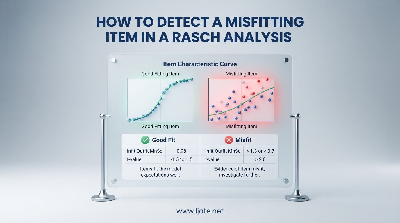
Rasch analysis is one of the most powerful tools in modern psychometrics for building and validating measurement instruments. But every Rasch practitioner eventually faces the same challenge: items that do not behave the way the model expects. If you are learning how to detect a misfitting item in a Rasch analysis, this guide walks you through every method, threshold, and decision point you need. We cover infit and outfit statistics, item-restscore correlations, simulation-based cutoffs, dimensionality checks, and a practical step-by-step workflow you can apply immediately.

Our team has spent years working with Rasch models across educational testing, health outcome instruments, and psychological scales. We have read the simulation studies from pgmj.github.io, the foundational work at rasch.org, the Winsteps documentation, and countless forum threads from r/psychometrics and the Rasch community boards. What we found is a gap between theory and practice that this guide closes. Most resources explain what fit statistics are but never tell you exactly what to do with them.

Before diving in, it helps to understand the Rasch model itself. The Rasch model is a probabilistic model that places person ability and item difficulty on the same logit scale. When data fits the model, you get interval-level measurement from ordinal responses. Researchers often start by comparing classical test theory and item response theory for item analysis before committing to a Rasch approach. The Rasch model’s strict requirements are what make misfit detection so important, because even one bad item can distort the entire measurement framework.

What Is a Misfitting Item in Rasch Analysis?

A misfitting item is an item whose observed response pattern deviates significantly from what the Rasch model predicts based on estimated person and item parameters. In simpler terms, the item does not measure the same latent trait as the rest of the scale, or it measures it in a way that introduces noise rather than signal. Misfit can mean the item is too unpredictable, too predictable, or tapping into a different dimension entirely.

Misfit matters because it directly threatens measurement quality. A single misfitting item can bias person ability estimates, reduce reliability, and undermine the construct validity of your instrument. In educational testing, this might mean a test question that advantages students for reasons unrelated to the measured ability. In health outcomes, it could mean a questionnaire item that patients interpret differently depending on cultural or linguistic factors.

There are two broad categories of misfit you will encounter. Underfit means the item is too noisy and unpredictable, contributing less information than the model expects. Overfit means the item is too predictable, often because it is redundant with other items or measures a narrower construct than intended. Both types degrade measurement, though underfit is generally more damaging.

How to Detect a Misfitting Item in a Rasch Analysis: Quick 4-Step Process

If you need a fast answer, here is the core workflow our team recommends for detecting misfitting items in a Rasch analysis:

Step 1: Run your Rasch model (dichotomous or polytomous) and extract item-level fit statistics including infit MNSQ, outfit MNSQ, infit ZSTD, and outfit ZSTD for every item.

Step 2: Flag any item whose infit or outfit MNSQ falls outside the acceptable range for your test type. For high-stakes tests, use 0.7 to 1.3. For routine scales, use 0.5 to 1.5. Flag items with ZSTD values beyond plus or minus 2.0 as additional confirmation.

Step 3: Cross-check flagged items using the item-restscore method. This provides an independent perspective by examining whether each item correlates appropriately with the rest of the scale. If both methods agree, your confidence in the misfit diagnosis increases significantly.

Step 4: Remove the worst-fitting item one at a time, re-run the analysis, and repeat. Iterative removal prevents cascading misfit where removing one item creates artificial misfit in others. Stop when all remaining items fit within acceptable ranges or when further removal would compromise content validity.

This four-step process forms the backbone of practical Rasch item fit analysis. The sections below explain each component in detail.

Method 1: Infit and Outfit Mean Square Statistics

Infit and outfit statistics are the most widely used tools for detecting item misfit in Rasch analysis. Both are based on residuals, which are the differences between observed responses and the responses the Rasch model expects. Large residuals indicate that an item behaves differently from what the model predicts.

Both statistics come in two forms: the mean square (MNSQ) version and the z-standardized (ZSTD) version. Understanding the difference between them is essential for accurate interpretation.

What Is the Mean Square (MNSQ)?

The mean square statistic is the average of squared standardized residuals for an item. A MNSQ value of 1.0 indicates perfect fit. Values greater than 1.0 indicate underfit, meaning the item is less predictable than the model expects. Values less than 1.0 indicate overfit, meaning the item is more predictable than expected.

MNSQ values are easy to interpret because they have a direct ratio interpretation. An outfit MNSQ of 1.5 means the item has 50 percent more variation than the model predicts. An infit MNSQ of 0.7 means the item shows 30 percent less variation than expected.

What Is Z-Standardized Fit (ZSTD)?

The ZSTD statistic converts the MNSQ into a standard normal distribution with a mean of 0 and a standard deviation of 1. This allows you to assess statistical significance. ZSTD values beyond plus or minus 2.0 suggest significant misfit at approximately the 0.05 level.

However, ZSTD is highly sensitive to sample size. With large samples, even trivially small deviations from perfect fit can produce statistically significant ZSTD values. This is why most practitioners rely primarily on MNSQ values for practical decisions and use ZSTD as a secondary indicator.

What Is the Difference Between Infit and Outfit?

The key difference between infit and outfit lies in how they weight residuals. Infit is information-weighted, meaning it gives more importance to responses near the item’s difficulty level. This makes infit less sensitive to outliers and more sensitive to structural misfit in the central part of the response distribution.

Outfit is unweighted, meaning every residual contributes equally. This makes outfit more sensitive to unexpected responses from people far from the item’s difficulty, such as a low-ability person answering a very difficult item correctly. Outfit is therefore more vulnerable to lucky guesses, careless errors, and other off-target responses.

For most practical applications, infit is the more diagnostic statistic for identifying items that fundamentally fail to measure the construct. Outfit is useful for detecting items with outlier problems. When infit and outfit disagree, prioritize infit for structural misfit assessment and investigate outfit for response anomalies.

Acceptable Infit and Outfit Ranges

The most commonly cited acceptable ranges come from the work of Wright, Linacre, and others at the MESA Psychometric Laboratory. For high-stakes testing and certification exams, infit and outfit MNSQ should fall between 0.7 and 1.3. For routine survey instruments and rating scales, the acceptable range widens to 0.5 to 1.5.

These are rule-of-thumb values, not universal truths. The research from pgmj.github.io and the Springer article on item fit statistics both demonstrate that these fixed cutoffs can produce unacceptably high false positive rates with large samples. With sample sizes above 500, even items that fit well in theory may exceed these thresholds. This is why simulation-based approaches, covered later in this guide, are increasingly recommended.

What Infit and Outfit Values Indicate Misfit?

As a practical summary, infit or outfit MNSQ values above 1.5 indicate significant underfit that warrants attention. Values between 1.3 and 1.5 suggest moderate misfit worth investigating. Values below 0.5 indicate overfit, meaning the item is not contributing independent information. ZSTD values beyond plus or minus 2.0 provide statistical confirmation but should always be interpreted alongside MNSQ values, especially with large samples.

Method 2: Item-Restscore Correlation

The item-restscore method offers a complementary approach to infit and outfit statistics for detecting misfitting items. Instead of comparing observed responses to model-based expectations, it examines whether each item correlates appropriately with the overall scale score computed from all other items.

The process is straightforward. For each item, compute the total score from all other items (the restscore). Then calculate the correlation between the target item and the restscore. Items that measure the same latent trait should show strong positive correlations with the restscore. Items that tap into a different construct or have measurement problems will show weak or even negative correlations.

The item-restscore method has several advantages. It is intuitive, easy to explain to non-specialists, and does not depend on specific distributional assumptions. It also provides a different lens on item quality that can catch problems that infit and outfit miss, particularly for off-target items that are either much easier or much harder than the rest of the scale.

Research comparing the detection rates of infit, outfit, and item-restscore methods shows interesting patterns. The simulation studies from pgmj.github.io found that item-restscore detection rates are competitive with infit and outfit for certain types of misfit, particularly when the misfitting item measures a substantively different dimension. However, item-restscore can struggle with items that have extreme difficulty levels, because the restscore may not provide enough discriminating information at those ability levels.

Our recommendation is to use item-restscore as a cross-validation tool alongside infit and outfit. When all three methods flag the same item, you can be confident in the diagnosis. When they disagree, the disagreement itself is diagnostic and points you toward understanding why the item misfits.

Method 3: Simulation-Based and Conditional Fit Statistics

Rule-of-thumb cutoffs for infit and outfit statistics have been the standard for decades. But mounting evidence from simulation research suggests these fixed thresholds are unreliable across different sample sizes, test lengths, and item types. Simulation-based approaches offer a more principled alternative.

Why Fixed Cutoffs Fall Short

The core problem with fixed cutoffs like 0.7 to 1.3 is that the sampling distribution of fit statistics depends heavily on sample size and test length. With small samples, fit statistics have wide distributions, meaning even fitting items can exceed the cutoff by chance. With large samples, the distributions narrow, and even tiny deviations from perfect fit become statistically significant.

The Springer article on whether we can trust Rasch item fit statistics demonstrated that the unconditional outfit and infit statistics have means slightly below the expected value of 1.0, especially when the number of items is small. This systematic bias means that applying fixed cutoffs can lead to incorrect decisions about item fit, particularly in shorter tests.

Parametric and Nonparametric Bootstrap

Bootstrap methods address this problem by generating empirical sampling distributions for each item’s fit statistics. The parametric bootstrap works by simulating response data from the fitted Rasch model, re-estimating fit statistics on the simulated data, and building a distribution of expected fit values. You then compare your observed fit statistics to this empirical distribution rather than to fixed cutoffs.

The nonparametric bootstrap takes a different approach. Instead of simulating from the Rasch model, it resamples the observed data with replacement to build empirical distributions. This can be useful when you are concerned about whether the Rasch model itself is the right reference distribution.

The R packages easyRasch and iarm provide functions for computing simulation-based critical values. The pgmj.github.io research used these tools to demonstrate that simulation-based cutoffs significantly reduce false positive rates compared to rule-of-thumb values, especially for samples under 500.

Conditional Likelihood Ratio Test (Andersen LRT)

The Andersen likelihood ratio test is another conditional approach to assessing item fit. It works by splitting the sample into groups based on total score, estimating item parameters separately for each group, and testing whether the estimates are significantly different across groups.

If items fit the Rasch model, their difficulty estimates should be invariant across score groups. Significant differences indicate that the item behaves differently for people at different ability levels, which is a form of misfit. The Andersen LRT is particularly useful because it is a global test that can detect overall fit problems before you drill into individual item statistics.

For researchers working with polytomous items, the Partial Credit Model extends Rasch analysis to rating scales and Likert-type items. Our colleagues have found explanatory item response models for polytomous item responses useful for extending misfit detection to multi-category response formats.

Interpreting Misfit: Underfit vs Overfit

Detecting that an item misfits is only the first step. Understanding what type of misfit it shows and what caused it determines whether you should remove, revise, or retain the item.

Underfit: Too Much Noise

Underfit occurs when infit or outfit MNSQ values exceed 1.0, indicating the item is less predictable than the Rasch model expects. Common causes include items that measure a different construct, items affected by local dependence, items with ambiguous wording that different respondents interpret differently, and items where guessing or carelessness plays a large role.

Underfitting items are generally more damaging than overfitting ones because they add noise that degrades measurement precision. An item with outfit MNSQ of 2.0 is contributing twice as much noise as the model expects, which directly reduces the reliability of person measures. Our team treats any item with MNSQ above 1.5 as a serious candidate for removal or revision.

Overfit: Too Predictable

Overfit occurs when MNSQ values fall below 1.0, indicating the item is more predictable than expected. This often happens when items are highly redundant with other items on the scale. Two items that ask essentially the same question will both show overfit because they perfectly predict each other’s responses.

Overfitting items are less immediately harmful than underfitting ones, but they inflate reliability estimates artificially and reduce measurement efficiency. An overfitting item does not add new information; it simply echoes what other items already capture. In practical terms, removing overfitting items often has minimal impact on person measures while streamlining the instrument.

When to Remove Items vs Retain Them

The decision to remove or retain a misfitting item should never be based on statistics alone. Content validity is paramount. If an item represents a critical aspect of your construct that no other item covers, removing it would create a content gap even if it improves statistical fit. In such cases, consider revising the item wording or format rather than eliminating it entirely.

As a general rule, our team removes items when their infit or outfit MNSQ exceeds 1.5 and they are not uniquely important for content coverage. We revise items with moderate misfit (1.3 to 1.5) that cover essential content. We retain items with borderline fit if removing them would reduce content validity or if the sample size is too small to trust the fit estimates.

For assessments involving multiple facets such as raters, tasks, and examinees, many-facet Rasch analysis for assessing rater effects provides additional tools for diagnosing whether misfit originates from items, raters, or interactions between them.

Step-by-Step Workflow for Iterative Item Removal

One of the biggest gaps in existing resources is practical guidance on the iterative process of removing misfitting items. Forum users on r/psychometrics and raschforum.boards.net consistently ask when to stop removing items and how to avoid cascading misfit. Here is the workflow our team uses.

Step 1: Initial Analysis

Run your full Rasch model with all candidate items. Extract infit MNSQ, outfit MNSQ, infit ZSTD, and outfit ZSTD for every item. Also compute item-restscore correlations for cross-validation. Document all values in a spreadsheet so you can track how fit statistics change as you remove items.

Step 2: Identify the Worst-Fitting Item

Sort items by their most extreme fit statistic. The item with the highest infit or outfit MNSQ above your threshold is your first candidate for removal. If multiple items show similarly severe misfit, investigate whether they share a common cause such as local dependence or multidimensionality.

Step 3: Remove One Item at a Time

Remove only the single worst-fitting item, then re-run the analysis. This is critical. Removing multiple items simultaneously can create artificial misfit in remaining items because the latent trait definition shifts when items are removed. One-at-a-time removal lets you observe the causal effect of each removal.

Step 4: Re-examine All Fit Statistics

After each removal, check whether previously fitting items have become misfitting. This can happen when the removed item was masking problems in other items or when the removal shifts the scale’s center of gravity. If previously fitting items suddenly misfit, stop and investigate the structural cause before continuing.

Step 5: Check Dimensionality

Periodically run PCA of residuals and Yen’s Q3 analysis to check for multidimensionality and local dependence. Sometimes what looks like item misfit is actually a multidimensional scale trying to split into two dimensions. Addressing dimensionality issues may resolve apparent misfit without item removal.

Step 6: Apply Stopping Rules

Continue the iterative process until all remaining items fit within acceptable ranges, or until further removal would compromise content validity. A practical stopping rule is to stop when removing the next-worst item would drop your reliability below an acceptable threshold or would leave you with too few items to adequately sample the construct.

For practitioners, we recommend documenting each iteration with the reason for each removal decision. This documentation supports the defensibility of your final instrument and helps reviewers understand your analytical process.

Sample Size Considerations

Sample size profoundly affects misfit detection accuracy. With samples below 100, fit statistics have wide sampling variability, meaning you will miss genuinely misfitting items (low detection power) and occasionally flag fitting items (false positives). With samples above 500, ZSTD values become hypersensitive, flagging trivially small deviations as significant.

The pgmj.github.io simulation research recommends different strategies based on sample size. For samples under 500, use simulation-based critical values rather than fixed cutoffs, and supplement with item-restscore correlations for additional evidence. For samples above 500, rely primarily on MNSQ values rather than ZSTD, and consider whether flagged items represent substantively meaningful misfit or just statistical artifacts of large sample size.

Detecting Multidimensionality and Local Dependence

Item misfit sometimes signals a deeper structural problem with your scale. Multidimensionality occurs when items measure more than one latent trait, violating the Rasch model’s unidimensionality assumption. Local dependence occurs when item responses are correlated for reasons beyond the shared latent trait, such as items that share a common passage or context.

PCA of Residuals

Principal component analysis of residuals examines the structure that remains after the Rasch model has extracted the primary dimension. If the residuals contain a strong secondary dimension, this suggests multidimensionality. Most Rasch software packages produce a PCA of residuals table showing the variance explained by the first contrast and the eigenvalue of the first residual component.

As a guideline, an eigenvalue of 2.0 or greater for the first residual contrast suggests a secondary dimension strong enough to contain at least two items. When you see this, examine which items load most strongly on the secondary dimension and consider whether they represent a meaningful subconstruct.

Yen’s Q3 Statistic

Yen’s Q3 measures the residual correlation between pairs of items after fitting the Rasch model. High residual correlations indicate local dependence, meaning the item pair shares variance beyond what the latent trait explains. A common cutoff is 0.20 above the mean residual correlation, though this varies with test length.

Local dependence can both cause and mask item misfit. Two locally dependent items may both show acceptable fit because they predict each other’s residuals, but together they violate the assumption of conditional independence. Alternatively, local dependence can create artificial misfit in non-dependent items by distorting the latent trait estimate.

For educational assessments, multidimensionality and item-level bias often require specialized detection methods. Our colleagues have demonstrated differential item functioning analysis using Rasch tree methods as an effective approach for identifying items that behave differently across demographic groups.

Common Mistakes in Rasch Misfit Detection

After reviewing forum discussions and analyzing the most common practitioner errors, we have identified several mistakes that compromise Rasch misfit detection. Avoiding these will significantly improve the quality of your analysis.

Mistake 1: Relying Solely on ZSTD Values

Because ZSTD is so sensitive to sample size, using it as your primary misfit criterion leads to false positives with large samples and false negatives with small samples. Always interpret ZSTD alongside MNSQ values, and prioritize MNSQ for practical decisions. ZSTD should confirm what MNSQ suggests, not drive the analysis.

Mistake 2: Applying Fixed Cutoffs Universally

The 0.7 to 1.3 range works reasonably well for moderate sample sizes and typical test lengths. But applying it blindly to samples of 50 or 5,000 leads to incorrect decisions. With small samples, relax your thresholds and use simulation-based cutoffs. With large samples, tighten your substantive interpretation and ask whether the misfit is practically meaningful, not just statistically significant.

Mistake 3: Removing Multiple Items Simultaneously

Bulk item removal saves time but destroys your ability to understand causal relationships. When you remove five items at once and fit improves, you cannot know which item was responsible. Worse, bulk removal can create artificial misfit in remaining items that then appear problematic. Always remove one item at a time, re-run the analysis, and document the effect of each removal.

Mistake 4: Confusing Item Misfit and Person Misfit

Person misfit and item misfit are distinct diagnostic concepts. Person misfit identifies respondents whose answer patterns deviate from model expectations, possibly due to guessing, carelessness, or fatigue. Item misfit identifies problems with specific questions. Confusing the two leads to incorrect remediation. Before removing an item, check whether person misfit is driving the item-level statistics. A small number of highly aberrant respondents can make an otherwise acceptable item appear to misfit.

Mistake 5: Ignoring Content Validity

Statistical fit is necessary but not sufficient for a defensible instrument. Removing items solely because of statistical misfit can strip your scale of content coverage. Every removal decision should weigh statistical evidence against content considerations. If a misfitting item is the only one covering a critical content area, revise rather than remove it.

Mistake 6: Stopping Too Early or Too Late

Stopping too early leaves misfitting items in the scale that degrade measurement. Stopping too late removes marginally fitting items that contribute meaningfully to content coverage. The iterative process requires judgment. Our team uses reliability indices, content coverage maps, and person separation statistics as complementary stopping criteria alongside fit thresholds.

Software Tools for Rasch Misfit Detection

Several software packages support Rasch analysis and item fit detection. Each has strengths and produces output in different formats, but all compute the core statistics you need.

Winsteps and Facets

Winsteps is the most widely used dedicated Rasch analysis software. It provides comprehensive item fit tables showing infit MNSQ, outfit MNSQ, infit ZSTD, and outfit ZSTD for every item. The Facets extension handles many-facet Rasch models for rater-mediated assessments. Winsteps output is well-documented and the website provides extensive guidance on interpreting fit statistics.

R Packages: eRm, iarm, and easyRasch

For researchers who prefer open-source tools, R offers several packages for Rasch analysis. The eRm package provides conditional maximum likelihood estimation for dichotomous and polytomous Rasch models. The iarm package specializes in item analysis and offers simulation-based fit statistics. The easyRasch package, developed alongside the pgmj.github.io research, implements parametric bootstrap methods for computing simulation-based critical values.

Forum users on r/rstats and r/psychometrics frequently ask for Winsteps alternatives. These R packages provide comparable functionality with the added benefits of reproducibility, script-based workflows, and no licensing costs. The learning curve is steeper than Winsteps, but the flexibility is greater for researchers who need custom analyses.

RUMM2030 and ConQuest are additional commercial options that offer unique features. RUMM2030 is known for its item-trait interaction statistics, which provide a global fit assessment. ConQuest supports multidimensional and multicomponent Rasch models for complex assessment structures.

Person Fit vs Item Fit: Understanding the Distinction

Throughout this guide we have focused on item fit, but person fit is an equally important diagnostic in Rasch analysis. Person fit statistics identify respondents whose answer patterns deviate from model expectations. The foundational work at rasch.org on diagnosing person misfit identifies several sources of idiosyncratic responses including guessing on multiple-choice items, carelessness on easy items, curriculum effects where respondents have learned specific content differently, and special knowledge that gives certain respondents unexpected advantages.

Person misfit and item misfit interact in important ways. A small number of highly aberrant respondents can inflate outfit statistics for items where their unexpected responses occur. Before removing an apparently misfitting item, examine person fit statistics to determine whether a few aberrant respondents are driving the item-level misfit. If so, consider whether those respondents should be retained or whether their responses reflect data quality issues.

For person fit assessment, infit is generally preferred over outfit because it is less sensitive to the extreme residuals that naturally occur at the tails of the ability distribution. The rasch.org guidance recommends focusing on infit for identifying persons whose response patterns fundamentally contradict the measurement model, while using outfit to flag persons with specific anomalous responses that may warrant investigation.

How to Detect a Misfitting Item in a Rasch Analysis: FAQ

Conclusion

Detecting a misfitting item in a Rasch analysis requires combining multiple statistical methods with substantive judgment about your construct and content. Start with infit and outfit MNSQ values as your primary diagnostic tool. Cross-validate with item-restscore correlations. Use simulation-based cutoffs when sample sizes are small or when fixed thresholds produce implausible results. Check dimensionality with PCA of residuals and Yen’s Q3 to ensure apparent item misfit is not masking a deeper structural problem.

The iterative process of removing one item at a time, re-running the analysis, and documenting each decision is what separates rigorous Rasch practice from mechanical application of cutoff values. Always balance statistical evidence against content validity, and remember that the goal is not perfect fit but a defensible, valid, and reliable measurement instrument. With the methods, thresholds, and workflow described in this guide, you have everything you need to detect and address misfitting items confidently in your Rasch analysis work.