What Infit and Outfit Mean in Rasch Measurement in (2026)?

If you have ever run a Rasch analysis and stared at a column of fit statistics wondering whether your items are performing well, you are not alone. Researchers, graduate students, and psychometricians routinely ask the same question: what exactly do infit and outfit mean in Rasch measurement, and how should I interpret them?

These two statistics are the most widely reported diagnostics in Rasch modeling. They tell you whether your data actually conforms to the model you are using to measure latent traits like ability, attitude, or severity of symptoms. Without checking fit, you cannot be confident that your measurement scale is working the way it should.

In this guide, I will walk you through clear definitions of infit and outfit, explain mean-square and standardized versions of each statistic, share interpretation guidelines with practical cutoff values, and provide examples of what misfit looks like in real research. I will also cover when to prioritize one statistic over the other, which is something most competing resources leave out.

For an applied example of Rasch analysis in practice, you can explore this empirical study on statistical adjustment of rater bias using Rasch analysis, which reports infit and outfit indices within recommended ranges.

What Is the Rasch Model?

The Rasch model is a psychometric framework for constructing measurement scales from categorical response data. It was developed by Danish mathematician Georg Rasch in the 1960s and has since become foundational in educational testing, health outcomes research, and social science measurement.

At its core, the model places both person ability and item difficulty on the same linear scale. A person with higher ability should have a higher probability of answering a given item correctly or endorsing a more difficult rating category. The model predicts the probability of each response based on the distance between the person’s ability and the item’s difficulty.

When real data matches those predictions, we say the data fits the model. When responses deviate systematically from what the model expects, we have evidence of misfit. That is where infit and outfit enter the picture.

The Rasch model assumes unidimensionality, meaning a single latent trait explains the pattern of responses. It also assumes local independence, where responses to different items are not correlated beyond what the latent trait accounts for. Fit statistics help you check whether these assumptions hold for your dataset.

Researchers use software like Winsteps, R packages such as TAM and eRm, or ConQuest to estimate Rasch models and produce fit statistics. Regardless of the software, the interpretation of infit and outfit follows the same principles I will describe below.

What Infit and Outfit Mean in Rasch Measurement

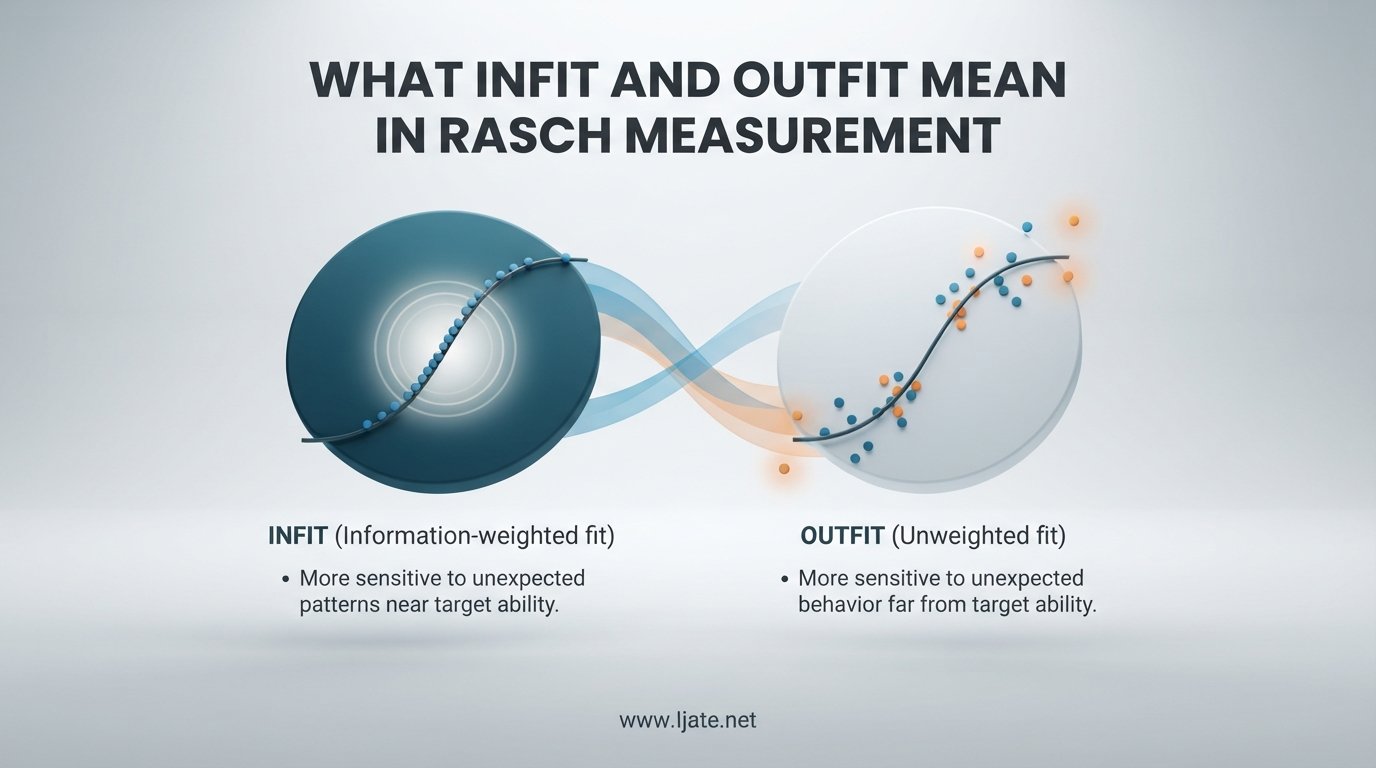
Infit means inlier-sensitive or information-weighted fit. Outfit means outlier-sensitive fit. Both are fit statistics that evaluate how accurately and predictably your data conform to the Rasch model, but they approach the question from different angles.

Every time a person responds to an item, there is a difference between what the model predicted and what actually happened. That difference is called a residual. Fit statistics summarize all those residuals across every person-item encounter into a single number for each item, and also for each person.

The key distinction is how each statistic handles those residuals. Infit gives more weight to responses that are close to what the model expected, meaning responses from people whose ability is near the item’s difficulty. Outfit treats every residual equally, regardless of whether the response was expected or surprising, which makes it especially sensitive to unexpected responses from people far above or below the item’s difficulty.

Think of it this way. If a moderately difficult item is answered correctly by a moderately able person, that is an inlier response, and infit pays close attention to it. If a very easy item is answered incorrectly by a very high-ability person, that is an outlier response, and outfit will flag it prominently.

Both statistics are reported in two forms: mean-square values and standardized values. I will explain each in detail in the sections that follow.

Infit Explained: How Information-Weighted Fit Works

Infit, formally called the information-weighted fit statistic, is designed to be sensitive to inliers. An inlier is a response where the person’s ability level is close to the item’s difficulty level. These are the responses that carry the most measurement information because they are right at the boundary of what the person can and cannot do.

The infit statistic calculates the average of squared residuals, but it weights each residual by its statistical information. Responses near the threshold of the person’s ability contribute more to the calculation, while responses that are far from the threshold contribute less. This makes infit a stable and reliable indicator of item performance for the typical range of respondents.

Because of this weighting, infit is less affected by off-target responses. If a low-ability person accidentally answers a very difficult item correctly, or a high-ability person carelessly misses a very easy item, infit will not overreact. Those outlier responses get small weights and have minimal influence on the infit value.

This is why most Rasch practitioners consider infit the primary diagnostic for item quality. It tells you whether the item is functioning as intended for the people it is designed to measure. If infit is too high, the item is producing noisy or unpredictable responses from people in its target range. If infit is too low, the item may be redundant or overly predictable, contributing little new information.

A common scenario in educational testing illustrates this well. Imagine a mathematics item calibrated at a difficulty of 0.5 logits. Students with abilities between 0.0 and 1.0 logits are the ones whose responses are most informative for evaluating this item. If those students respond unpredictably, some getting it right and some wrong in ways the model cannot account for, infit will rise above 1.0, signaling potential problems with the item.

Outfit Explained: How Outlier-Sensitive Fit Works

Outfit, formally called the outlier-sensitive fit statistic, takes a different approach. It computes the average of squared residuals without applying any information weights. Every person-item interaction contributes equally to the outfit value, regardless of how far the person’s ability is from the item’s difficulty.

This unweighted approach makes outfit highly sensitive to outliers. A single unexpected response from a person whose ability is very different from the item’s difficulty can inflate the outfit statistic significantly. This sensitivity can be both a strength and a limitation depending on your research context.

On the positive side, outfit is excellent for detecting carelessness, guessing, or other aberrant response patterns. If a high-ability test-taker misses an extremely easy item, outfit will catch it. If a low-ability test-taker guesses correctly on a hard item, outfit will flag that too. These are exactly the kinds of anomalies you want to identify when cleaning data or diagnosing measurement problems.

On the negative side, outfit can overreact to small numbers of extreme responses. With large samples, even a few off-target respondents can push outfit values above acceptable thresholds without indicating any real problem with the item itself. This is why researchers often treat high outfit values with caution and investigate them in context before making decisions about item removal.

In clinical and health outcome measurement, outfit is particularly useful for identifying respondents who may have misunderstood instructions, answered randomly, or had unusual response patterns due to fatigue or attention loss. A person-level outfit value above 2.0 often triggers a closer look at that individual’s response pattern.

It is worth noting that outfit tends to be more variable than infit across different samples and testing conditions. For this reason, many methodologists recommend reporting both statistics but giving more weight to infit when making decisions about item retention or revision.

Mean-Square Fit Statistics: Size of the Distortion

The mean-square version of infit and outfit, often abbreviated as MNSQ, shows the size of the randomness in your data. It quantifies how much distortion exists in the measurement system for each item or person. The expected value for both infit MNSQ and outfit MNSQ is 1.0 when the data perfectly fits the Rasch model.

A mean-square value of 1.0 means the observed variance in residuals matches what the model predicts. Values above 1.0 indicate more variation than expected, meaning the item or person is less predictable than the model assumes. Values below 1.0 indicate less variation than expected, meaning responses are more deterministic than the model predicts.

Here is a practical interpretation guide for mean-square fit values that draws from guidelines established by Richard Smith and John Linacre, two of the most frequently cited authorities in Rasch methodology:

• 0.5 to 1.5: Productive measurement. The item or person contributes useful information to the measurement system. No action needed.

• 1.5 to 2.0: Unproductive but not degrading. The item may add noise but does not distort the measure. Review for potential improvement.

• Greater than 2.0: Degrades the measurement system. The item or person adds enough noise to distort the measurement and should be flagged for revision or removal.

• Less than 0.5: Overly predictable. The item may be redundant or the person may have a response pattern that is too narrow to contribute meaningful information.

These ranges serve as general benchmarks, not absolute rules. Some researchers use tighter cutoffs for high-stakes assessments and looser cutoffs for exploratory scale development. The key is to interpret mean-square values in the context of your specific instrument, sample, and research goals.

It is also important to understand that mean-square values are not sample-size dependent in the same way significance tests are. A mean-square of 1.3 means roughly the same thing whether you have 100 or 1,000 respondents. This stability is one reason practitioners often prefer mean-square values over standardized statistics for routine item evaluation.

Standardized Fit Statistics: Zstd and t-Values

While mean-square statistics tell you the size of misfit, standardized fit statistics tell you whether that misfit is statistically significant. The standardized version, often labeled Zstd or t, converts the mean-square value into a t-statistic using a Wilson-Hilferty transformation of the chi-square distribution.

The expected value for standardized fit statistics is 0. Values above 0 indicate more misfit than expected, and values below 0 indicate less misfit than expected. As a general rule, standardized values beyond positive or negative 2 suggest statistically significant misfit at approximately the 0.05 level.

Here is the critical caveat that many researchers miss. Standardized statistics are highly sensitive to sample size. With very large samples, even trivially small deviations from perfect fit can produce Zstd values beyond plus or minus 2. With small samples, substantial misfit may not reach significance because the test lacks statistical power.

This sample-size sensitivity creates a common trap. A researcher with 2,000 respondents sees several items with Zstd values of 3 or 4 and assumes those items are seriously flawed. In reality, the mean-square values may be 1.1 or 1.2, well within the productive range. The standardized statistic is flagging statistical significance, not practical significance.

For this reason, most experienced Rasch analysts prioritize mean-square values for substantive interpretation and use standardized statistics as a secondary check. When both MNSQ and Zstd point in the same direction, you can be confident in your assessment. When they disagree, trust the mean-square for practical decisions.

Some software packages, including Winsteps, report standardized values with a notation indicating they are approximations rather than exact probabilities. This is because the distribution of fit statistics under the Rasch model is not perfectly normal, especially for items answered by small numbers of people or for persons who answered very few items.

Infit vs Outfit: When to Prioritize Each

One of the most common questions in Rasch forums and graduate seminars is whether to prioritize infit or outfit when evaluating items and persons. The answer depends on what you are trying to detect and the characteristics of your sample.

For routine item evaluation, infit should be your primary diagnostic. Because it is weighted by information and resistant to outlier distortion, infit provides a stable estimate of how well an item functions for respondents in its target difficulty range. When infit values fall between 0.5 and 1.5, you can be reasonably confident that the item is contributing productively to measurement.

Outfit becomes more important when you are conducting data quality checks. If you suspect that some respondents guessed, answered carelessly, or had comprehension issues, outfit will surface those problems. A person with an outfit MNSQ above 2.0 deserves a closer look at their response pattern to determine whether their data should be retained or excluded.

For polytomous data, such as Likert-scale responses, both statistics matter but infit tends to be more informative about the structure of the rating scale. High infit on polytomous items can indicate that respondents are using the categories inconsistently or that the category thresholds are disordered.

Sample size plays a role too. With small samples, outfit values can swing dramatically due to a single unexpected response. In those cases, do not overinterpret outfit. With very large samples, outfit values tend to stabilize, and high outfit more reliably indicates a genuine problem.

A practical decision framework looks like this. Start by reviewing infit MNSQ for all items. Flag anything above 1.5 for closer inspection. Then check outfit MNSQ for flagged items and for all persons. Items with both high infit and high outfit are the strongest candidates for revision or removal. Items with high outfit but normal infit may be fine if the sample contains many off-target respondents.

How to Interpret Infit and Outfit Values: A Practical Guide

Let me walk you through a concrete example to show how interpretation works in practice. Suppose you are analyzing a 20-item reading comprehension test administered to 500 students. After running the Rasch model in Winsteps, you examine the item fit table.

Item 7 shows an infit MNSQ of 0.98, an outfit MNSQ of 1.05, an infit Zstd of 0.3, and an outfit Zstd of 0.5. All values are close to their expected values. This item fits the model well and is functioning as intended.

Item 12 shows an infit MNSQ of 1.78, an outfit MNSQ of 2.31, an infit Zstd of 4.2, and an outfit Zstd of 5.1. Both mean-square values exceed the productive range, and both standardized values are well beyond 2. This item is seriously misfitting and likely degrading the measurement system. You should examine the item content, check for ambiguous wording or double-keyed answers, and consider revising or removing it.

Item 15 shows an infit MNSQ of 1.12, an outfit MNSQ of 1.85, an infit Zstd of 1.1, and an outfit Zstd of 3.0. Infit is within range, but outfit is elevated. This pattern suggests the item works well for students near its difficulty level but produces some unexpected responses from students far above or below that level. You might retain the item but investigate whether extreme groups are interpreting it differently.

When you encounter misfitting items, several remedies are available. You can revise the item wording to improve clarity. You can check whether the item is multidimensional, which would violate the unidimensionality assumption. You can examine item characteristic curves to visualize where the misfit occurs. Or you can remove the item entirely if revision is not feasible.

For person fit, the same interpretation logic applies. A person with high outfit MNSQ may have guessed, rushed, or misread items. Their measure may still be usable, but it should be interpreted with caution. A person with high infit MNSQ is responding unpredictably even on items matched to their ability level, which raises more serious concerns about the validity of their score.

Remember that fit statistics are diagnostic tools, not automatic decision rules. Always consider the substantive content of items, the characteristics of your sample, and the purpose of your measurement instrument before removing items or excluding persons based solely on fit values.

FAQs

Conclusion

Understanding what infit and outfit mean in Rasch measurement is essential for anyone working with psychometric instruments. Infit gives you a stable, information-weighted view of how well items function for their target respondents. Outfit helps you catch outliers and aberrant response patterns that could compromise data quality.

Both statistics come in mean-square and standardized forms. Mean-square values tell you the practical size of any misfit, with 0.5 to 1.5 being the productive range and anything above 2.0 degrading your measurement. Standardized values add statistical significance but should be interpreted cautiously with large samples.

When you sit down to evaluate your next Rasch analysis output, start with infit MNSQ as your primary diagnostic, check outfit for data quality issues, and remember that fit statistics are tools to guide judgment, not replace it. The next step is to apply these guidelines to your own data and see what patterns emerge.