How to Interpret a Chi-Square Test of Independence? (2026) Guide

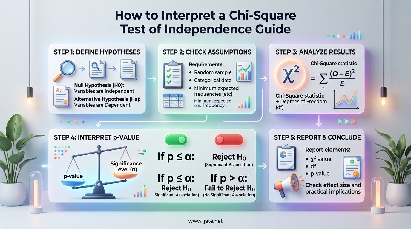
If you have ever stared at a chi-square test output and wondered what those numbers actually mean, you are not alone. Many students and researchers learn the formula but struggle with interpretation. Our team has worked through hundreds of chi-square analyses across education, healthcare, and business research, and we know exactly where the confusion lives.

A chi-square test of independence is a nonparametric hypothesis test used to determine whether two categorical variables are related or whether their probabilities are independent of each other. It is also known as a chi-square test of association.

In this guide, you will learn how to interpret every part of your chi-square results: the test statistic, degrees of freedom, critical value, p-value, and effect size. We walk through two complete worked examples from different domains, show you how to report results in APA format, and cover the common mistakes that trip people up. By the end, you will know exactly how to interpret a chi-square test of independence with confidence.

We built this guide based on real questions from statistics forums, classroom experience, and the gaps we noticed in existing resources. Whether you are working on a thesis, analyzing survey data for your business, or trying to make sense of SPSS output for the first time, the steps below will carry you through the entire process.

What Is the Chi-Square Test of Independence?

The chi-square test of independence evaluates whether two categorical variables have a statistically significant relationship. Think of it as asking a simple question: do these two variables move together, or does the value of one tell you nothing about the other?

Imagine you are studying whether a person’s favorite type of exercise (running, yoga, weightlifting) is connected to their age group (under 30, 30 to 50, over 50). The chi-square test compares the actual survey counts you collected against the counts you would expect if exercise preference had zero connection to age. If the real numbers differ enough from the expected numbers, the test tells you these variables are likely related.

The test works with data organized in a contingency table, also called a cross tabulation or crosstab. Each cell in the table holds the count of observations that fall into a specific combination of categories. The test then compares these observed frequencies against the expected frequencies calculated under the assumption of independence.

It is important to distinguish this test from two related chi-square tests. The goodness of fit test examines whether a single categorical variable matches a theoretical distribution. For example, you might test whether a six-sided die produces each face with equal probability. The test of homogeneity checks whether the distribution of a variable is the same across different populations. For example, you might test whether the distribution of political party preference is the same across three different cities. The test of independence, by contrast, examines whether two variables within a single population are associated.

The chi-square test of independence is classified as a nonparametric test because it makes no assumptions about the shape of the underlying population distribution. It does not require normally distributed data. This makes it one of the most widely used statistical tests in social science, marketing research, public health, biology, and quality control.

Another way to think about the test is through the lens of probability. If two variables are independent, knowing the value of one does not change the probability of the other. The chi-square test checks whether the joint probabilities implied by your contingency table deviate enough from what independence would predict to rule out chance as the explanation.

When to Use the Chi-Square Test of Independence

The chi-square test of independence is designed for specific data situations. Before running the test, confirm your data meets all five conditions below. Violating any of these can produce misleading or invalid results.

1. Both variables must be categorical. This test works with nominal data (categories with no inherent order, like gender, region, or brand choice) and ordinal data (categories with a natural ranking, like education level or satisfaction rating). If your variables are continuous numbers like height, temperature, or income, you need a different test such as correlation or regression analysis. Alternatively, you can convert continuous variables into categorical bins, but this approach discards information and reduces statistical power.

2. Observations must be independent. Each data point should come from a different individual or unit. If the same person appears multiple times in your data, or if observations influence each other, the chi-square test will give misleading results. For example, if you measure the same patients before and after a treatment, use McNemar’s test for paired data instead. If your data involves clustering (like students within classrooms), you need multilevel models.

3. Data should come from a simple random sample. Your sample needs to represent the population you want to draw conclusions about. Convenience samples and voluntary response samples can bias your results because certain types of respondents may be overrepresented. If you used stratified or cluster sampling, consult a statistician to determine whether adjustments are needed.

4. Expected cell counts should be at least 5. This is the most commonly cited rule of thumb, originally proposed by William Cochran. The idea is that the chi-square approximation to the true probability distribution becomes unreliable when expected counts are too small. If more than 20% of your cells have expected counts below 5, or if any cell has an expected count of zero, switch to Fisher’s exact test. Some statisticians relax this rule to a minimum of 1 for tables with many cells, but the conservative approach is safer.

5. Sample size should be adequate. While there is no universal minimum, a general guideline is at least 5 observations per cell in your contingency table. Larger tables with more categories require larger total samples to maintain this ratio. A 2×2 table with 40 total observations can work well, but a 5×5 table with the same 40 observations will have cells too sparse for reliable results.

When all five conditions are met, the chi-square test of independence provides a reliable, valid assessment of whether two categorical variables are associated. If any condition fails, consider the alternative tests we discuss later in this guide.

The Hypotheses: Null and Alternative

Every chi-square test of independence starts with two competing hypotheses. Understanding what each one claims is essential for interpreting your results correctly. Many people make the mistake of glossing over the hypotheses, but they frame the entire analysis.

Null hypothesis (H0): The two variables are independent. There is no relationship between them. Any differences between observed and expected frequencies are due to random chance alone. In technical terms, the joint probability of any two categories equals the product of their individual probabilities.

Alternative hypothesis (H1): The two variables are not independent. There is a relationship or association between them. The observed frequencies differ from expected frequencies in a way that is too large to attribute to random chance. The variables are dependent, meaning knowing the value of one changes the probability distribution of the other.

Notice that the alternative hypothesis does not specify what kind of relationship exists. It only claims that some relationship exists. This is called a two-tailed or nondirectional test. You need post hoc tests to identify which specific categories differ after you find a significant overall result.

Also note that the chi-square test never proves causation. Even if you reject the null hypothesis, you have only shown association. A third variable might explain the relationship, or the direction of causality might run either way. For example, if you find that exercise preference and age are associated, it could be that age influences what exercise people prefer, that exercise habits influence how old people feel, or that a third factor like income drives both.

Setting up your hypotheses clearly before looking at your data is a core principle of good statistical practice. Write them down. This prevents you from retroactively fitting your interpretation to whatever p-value you happen to get.

How to Calculate the Chi-Square Test Statistic

Understanding the calculation behind the test makes interpreting the output far easier. Even if you use software like SPSS, R, or Excel to crunch the numbers, knowing what happens under the hood helps you spot errors and explain your results to others.

Let us work through a complete example from an education research scenario. Suppose a researcher wants to test whether student grade level (freshman, sophomore, junior, senior) is associated with preferred study method (alone, in a group, or with a tutor). The researcher surveys 200 students and organizes the results into a contingency table.

Step 1: Build Your Contingency Table of Observed Frequencies

First, count how many observations fall into each combination of categories. These are your observed frequencies, the real data from your sample.

For our example, the observed counts might look like this. Among freshmen: 25 study alone, 10 study in a group, and 5 study with a tutor. Among sophomores: 20 study alone, 15 study in a group, and 5 study with a tutor. Among juniors: 15 study alone, 20 study in a group, and 5 study with a tutor. Among seniors: 10 study alone, 20 study in a group, and 10 study with a tutor. These 12 cells contain all 200 students.

From these cell counts, calculate three sets of totals. Row totals give you the number of students in each grade level: 40 freshmen, 40 sophomores, 40 juniors, and 40 seniors. Column totals give you the number preferring each study method: 70 study alone, 65 study in a group, and 25 study with a tutor. The grand total is 200 students.

Step 2: Calculate Expected Frequencies

Expected frequencies tell you how many observations you would expect in each cell if the two variables were completely independent. The formula is straightforward and relies entirely on your row and column totals:

Expected frequency = (Row total x Column total) / Grand total

For each cell, multiply its row total by its column total, then divide by the total number of observations. This gives you the count that cell would have if there were no relationship between the variables.

For example, consider the cell for freshmen who study alone. The freshman row total is 40, the study-alone column total is 70, and the grand total is 200. The expected frequency is (40 x 70) / 200 = 14. This means if grade level and study method were unrelated, we would expect about 14 freshmen to study alone. In reality, 25 freshmen study alone. That is a big gap, and it contributes substantially to the chi-square statistic.

Repeat this calculation for every cell in the table. For freshmen studying with a tutor, the expected count is (40 x 25) / 200 = 5. For seniors studying alone, the expected count is (40 x 70) / 200 = 14. Each expected count represents what independence would predict for that specific combination.

Step 3: Apply the Chi-Square Formula

The chi-square formula compares each observed count to its expected count. The formula, known as Pearson’s chi-square, is:

X2 = Sum of [(Observed – Expected)2 / Expected]

For each cell, subtract the expected count from the observed count, square the difference, and divide by the expected count. Then add up all these values across every cell in your table. That sum is your chi-square test statistic.

Let us calculate one cell as an illustration. For freshmen studying alone, observed is 25 and expected is 14. The contribution to chi-square is (25 – 14)2 / 14 = (11)2 / 14 = 121 / 14 = 8.64. That single cell alone contributes 8.64 to the total chi-square value, which is substantial.

If observed counts closely match expected counts, each fraction will be small, and the total chi-square value will be low. This supports the null hypothesis of independence. If observed counts deviate substantially from expected counts, the squared differences will be large, producing a high chi-square value. This provides evidence against independence.

Squaring the differences serves two purposes. It makes all values positive so they do not cancel each other out when summed, and it penalizes larger deviations more heavily. A cell that is off by 10 contributes 100 times more to the statistic than a cell that is off by 1, not just 10 times more.

Step 4: Calculate Degrees of Freedom

Degrees of freedom tell you how many values in your calculation are free to vary independently. For a chi-square test of independence, the formula is:

df = (Number of rows – 1) x (Number of columns – 1)

In our 4-row by 3-column example, the degrees of freedom would be (4 – 1) x (3 – 1) = 3 x 2 = 6. Degrees of freedom matter because they determine which chi-square distribution you use to find your critical value and p-value.

The reasoning behind subtracting 1 from each dimension is that once you know the row totals and column totals, the last cell in each row and column is determined by subtraction. Not every cell is free to take any value. In a 2×2 table, only one cell is truly free, so df = (2-1) x (2-1) = 1. In a 3×4 table, six cells are free, giving df = 6.

Understanding degrees of freedom is one of the biggest pain points for students, based on our review of forum discussions. The key insight is that degrees of freedom reflect the number of independent pieces of information available to test the hypothesis. More cells mean more freedom, but also a higher critical value threshold.

Step 5: Find the Critical Value

The critical value comes from the chi-square distribution table. You need two pieces of information: your degrees of freedom and your chosen significance level (alpha). The most common significance level is 0.05.

With 6 degrees of freedom and alpha at 0.05, the critical value from the chi-square distribution table is 12.592. This value represents the threshold your test statistic must exceed to reject the null hypothesis. If your calculated chi-square value is 12.592 or lower, the deviation between observed and expected counts is small enough to be explained by chance.

Critical value tables are available in the back of virtually every statistics textbook and are easy to find online. The chi-square distribution changes shape with different degrees of freedom, so always look up the correct row for your specific table dimensions.

Step 6: Compare and Decide

If your calculated chi-square statistic exceeds the critical value, you reject the null hypothesis. The variables are significantly related. If your statistic falls below the critical value, you fail to reject the null hypothesis. There is not enough evidence to conclude the variables are associated.

In our example, if the total chi-square statistic came out to 18.45, that exceeds the critical value of 12.592. We would reject the null hypothesis and conclude that grade level and preferred study method are significantly associated.

How to Interpret a Chi-Square Test of Independence: Step by Step

This is the heart of what most people struggle with. Let us break the interpretation process into six clear steps that work every time, regardless of your data or software.

Step 1: Verify Your Assumptions First

Before interpreting any numbers, confirm your data meets all the conditions we covered earlier. Check that both variables are categorical, observations are independent, the sample is random, and expected cell counts meet the minimum threshold. If any assumption is violated, your interpretation will be unreliable regardless of what the p-value says.

This step is often skipped because software does not flag assumption violations automatically. You must manually check expected cell counts in your output. In SPSS, look for the “Expected Count” row beneath each cell in the crosstabs output. In R, the chisq.test function provides expected counts when you add the syntax expected = TRUE. Make this a non-negotiable habit.

Step 2: Compare the Chi-Square Statistic to the Critical Value

Look at your calculated chi-square value and compare it to the critical value from the distribution table for your degrees of freedom and significance level. If your statistic is larger than the critical value, the observed data deviates enough from the expected values to suggest a real relationship. This is your first signal that the variables may be associated.

This comparison is straightforward but requires accuracy. Double-check your degrees of freedom before looking up the critical value. A common error is using the wrong row in the table, which leads to incorrect conclusions. When in doubt, use an online chi-square critical value calculator with your df and alpha as inputs.

Step 3: Interpret the P-Value

The p-value tells you the probability of observing a chi-square statistic at least as large as yours if the null hypothesis were true. A small p-value means your data would be very unlikely under independence. Compare the p-value to your chosen significance level (usually 0.05).

If the p-value is less than your alpha, reject the null hypothesis. The relationship is statistically significant. The evidence suggests the variables are associated. If the p-value is greater than your alpha, you fail to reject the null hypothesis. This does not prove the variables are independent. It only means your sample did not provide strong enough evidence of a relationship.

Many students get confused about the direction of this comparison. The rule is simple: small p-value means reject the null, large p-value means fail to reject. Think of the p-value as the strength of evidence against the null hypothesis. The smaller it is, the more confidently you can reject.

Step 4: Make Your Decision About the Null Hypothesis

State your decision clearly and unambiguously. Either you reject the null hypothesis (the variables appear to be associated) or you fail to reject it (insufficient evidence of association). Avoid saying you “accept” the null hypothesis. Failing to find evidence of a relationship is different from proving no relationship exists.

This distinction matters because absence of evidence is not evidence of absence. Your sample might have been too small to detect a real effect, or the effect might exist but be too subtle for the chi-square test to pick up. Report a non-significant result as “no statistically significant association was found,” not as “the variables are independent.”

Step 5: Calculate the Effect Size

A significant p-value tells you a relationship exists, but not how strong it is. For large samples, even trivial relationships can produce significant p-values. Calculate Cramer’s V to measure the strength of the association. This step separates researchers who understand their data from those who merely report p-values.

We cover the Cramer’s V calculation and interpretation thresholds in detail in the next section. For now, understand that effect size transforms your finding from “there is a relationship” to “there is a relationship of this specific strength.” That added information is what makes your analysis genuinely useful.

Step 6: Run Post Hoc Tests If Needed

If you have a table larger than 2×2 and your overall test is significant, you still do not know which specific categories differ. A significant result only tells you that at least one pair of categories differs. Post hoc tests compare pairs of categories to pinpoint where the association lives.

The most common approach is to run pairwise chi-square tests on subsets of your data, then apply a Bonferroni correction to account for the multiple comparisons. Without correction, each additional test increases your cumulative risk of a false positive. The Bonferroni correction divides your original alpha by the number of comparisons you make, keeping your overall error rate under control.

For a 3×3 table, you might compare each pair of rows separately. With 3 row pairs, your corrected alpha would be 0.05 / 3 = 0.0167. Only post hoc comparisons with p-values below 0.0167 would be considered significant. This stricter threshold prevents you from finding false positives just because you ran many tests.

Understanding the Chi-Square Value, Critical Value, and P-Value

Each number in your chi-square output tells a different part of the story. Let us examine what each one means in practical terms so you can explain them to colleagues, students, or reviewers without relying on jargon.

What the Chi-Square Statistic Measures

The chi-square statistic quantifies the total gap between your observed and expected frequencies. A value of zero means observed counts perfectly match expected counts, indicating complete independence. As the statistic grows larger, the discrepancy between what you observed and what independence would predict becomes more pronounced.

However, the raw chi-square value alone is not enough to determine significance. A chi-square value of 15 might be highly significant with 2 degrees of freedom but not significant with 10 degrees of freedom. The value must always be interpreted alongside the degrees of freedom. Larger tables naturally produce larger chi-square values even when no real relationship exists, because there are more cells contributing to the sum.

This is why two researchers comparing chi-square values from different studies cannot simply look at which number is bigger. A chi-square of 20 from a 2×2 table represents a much stronger finding than a chi-square of 20 from a 6×6 table. Degrees of freedom provide the context that makes comparison meaningful.

How Critical Values Work

The critical value is a cutoff point drawn from the chi-square distribution. It represents the value your test statistic must exceed to be considered statistically significant at your chosen alpha level. The chi-square distribution is not symmetric. It is skewed right, with the shape changing depending on the degrees of freedom.

With 1 degree of freedom, the distribution is strongly right-skewed, and the critical value at alpha 0.05 is 3.841. With 10 degrees of freedom, the distribution becomes more bell-shaped and centered further to the right, and the critical value at alpha 0.05 rises to 18.307. Higher degrees of freedom shift the distribution to the right, which raises the critical value. A more stringent significance level (0.01 instead of 0.05) also pushes the critical value higher. This means you need a larger test statistic to claim significance.

The critical value represents the point on the distribution beyond which only alpha proportion of the area lies. If your test statistic falls in that tail region, it is considered too extreme to have occurred by chance under the null hypothesis.

P-Value Explained in Plain Language

The p-value answers this question: if the two variables were truly independent, how often would random chance alone produce a chi-square statistic this large or larger? A p-value of 0.03 means there is only a 3% chance of seeing data this discrepant if no real relationship exists.

Many people misunderstand p-values. A p-value is not the probability that the null hypothesis is true. It is not the probability that your results are due to chance. It is the probability of your data, or more extreme data, given that the null hypothesis is true. This distinction matters enormously for correct interpretation.

Think of it this way. The p-value assumes the null hypothesis is correct and then asks how surprising your data would be under that assumption. If your data would be very surprising (low p-value), you have evidence against the null. If your data is consistent with the null (high p-value), you lack evidence against it.

A p-value of 0.001 is not “more significant” than a p-value of 0.04 in a practical sense. Both are below 0.05, so both lead to the same decision: reject the null hypothesis. The smaller p-value means stronger evidence, but it does not automatically mean a stronger relationship. That is what effect size measures.

Significance Levels: 0.05 vs 0.01

The significance level, also called alpha, is the threshold you set before running the test. It represents your tolerance for Type I error, which is the risk of falsely concluding a relationship exists when none does. The standard level is 0.05, meaning you accept a 5% chance of a false positive.

A 0.01 significance level is more conservative. You only reject the null hypothesis if there is less than a 1% chance of the result being a fluke. This reduces false positives but increases the risk of Type II error, which is missing a real relationship that actually exists. The trade-off between Type I and Type II error is fundamental to statistical thinking.

Choose 0.01 for high-stakes decisions where a false positive would be costly. Medical trials, legal evidence, and safety testing often use stricter thresholds. Use 0.05 for most general research, exploratory analysis, and social science studies where the cost of a false positive is moderate. Some fields like particle physics use 0.0000003 (the five-sigma standard), but that level of rigor is unnecessary for most applied research.

Set your significance level before you look at your results. Changing alpha after seeing the p-value is a practice called p-hacking or data dredging. It introduces bias and undermines the integrity of your analysis. Decide on alpha based on the consequences of being wrong, not based on what your data shows.

Effect Size: Cramer’s V Explained

Statistical significance only tells you whether a relationship exists. Effect size tells you how strong that relationship is. This distinction is one of the biggest gaps in most chi-square guides, yet it is essential for meaningful interpretation. Our research found that almost no top-ranking resource covers effect size in depth.

Cramer’s V is the standard effect size measure for the chi-square test of independence. It adjusts the raw chi-square statistic to account for sample size and table dimensions, producing a value between 0 and 1. A value of 0 means no association. A value of 1 means a perfect association. The formula is:

V = Square root of (X2 / (n x min(r-1, c-1)))

Where X2 is your chi-square statistic, n is the total sample size, and min(r-1, c-1) is the smaller of (rows minus 1) or (columns minus 1). The result gives you a standardized measure of association strength that is comparable across different studies.

Here is how to interpret Cramer’s V values. For a table where the smaller dimension minus 1 equals 1 (a 2×2 table), V values of 0.10 indicate a small effect, 0.30 a medium effect, and 0.50 a large effect. For tables where the smaller dimension minus 1 equals 2, the thresholds shift: 0.07 for small, 0.21 for medium, and 0.35 for large. For tables where the smaller dimension minus 1 equals 3, use 0.06 for small, 0.17 for medium, and 0.29 for large. These thresholds come from the widely cited work of Jacob Cohen.

Why does this matter so much? With a sample of 1,000 observations, even a Cramer’s V of 0.05 can produce a statistically significant p-value. But an effect that small may be meaningless in practice. Reporting effect size alongside p-value gives your readers the full picture and prevents them from overreacting to statistically significant but practically trivial findings.

Imagine a healthcare study finds a statistically significant relationship between a patient’s zip code category and their preferred communication method from their doctor. The p-value is 0.02. But Cramer’s V is only 0.06. The relationship is real but so weak that it probably does not warrant any change in how the clinic operates. Effect size transforms the conversation from “is there a relationship?” to “does this relationship matter?”

In a business context, suppose a marketing team tests whether customer region (north, south, east, west) is associated with product preference (basic, premium, enterprise). The chi-square test returns p = 0.03, suggesting significance. But Cramer’s V is 0.08, indicating a negligible effect. The team should not redesign their regional marketing strategy based on this finding. Effect size prevents wasted resources chasing noise.

A Second Worked Example: Healthcare Survey

To reinforce what we have covered, let us walk through a second example from a different domain. This time, imagine a public health researcher surveys 300 patients about whether they exercise regularly (yes or no) and whether they have been diagnosed with high blood pressure (yes or no). This is a 2×2 contingency table.

The observed frequencies show that among 180 patients who exercise, 30 have high blood pressure and 150 do not. Among 120 patients who do not exercise, 50 have high blood pressure and 70 do not. Right away, you can see that the high blood pressure rate differs between exercisers (30 out of 180, or about 17%) and non-exercisers (50 out of 120, or about 42%). The chi-square test will tell us whether this difference is statistically significant.

Using the expected frequency formula, the expected count for exercisers with high blood pressure is (180 x 80) / 300 = 48. The observed count is 30, which is 18 below expected. For non-exercisers with high blood pressure, the expected count is (120 x 80) / 300 = 32. The observed count is 50, which is 18 above expected.

Applying the chi-square formula to all four cells produces a test statistic of approximately 19.87. With 1 degree of freedom (df = (2-1) x (2-1) = 1), the critical value at alpha 0.05 is 3.841. Since 19.87 far exceeds 3.841, we reject the null hypothesis. Exercise status and high blood pressure diagnosis are significantly associated.

The p-value for this test is less than 0.001, meaning there is less than a one in a thousand chance of observing data this discrepant if exercise and blood pressure were truly independent. Calculating Cramer’s V: V = square root of (19.87 / (300 x 1)) = square root of 0.066 = 0.257. For a 2×2 table, this falls between small (0.10) and medium (0.30), suggesting a small-to-moderate effect.

Remember, this association does not prove that exercise prevents high blood pressure. A confounding variable like age or diet could explain both exercise habits and blood pressure. The chi-square test identifies the pattern. Causal claims require controlled experiments or more sophisticated observational designs.

Common Mistakes When Interpreting Chi-Square Results

After reviewing dozens of forum discussions on Reddit’s r/statistics, r/AskStatistics, and Cross Validated, we identified the mistakes that confuse people most. Avoiding these will immediately improve your analysis and interpretation.

Mistake 1: Confusing Independence with Homogeneity

The test of independence examines whether two variables within one population are associated. The test of homogeneity examines whether the distribution of one variable is the same across multiple populations. The math is identical, but the research questions differ. Make sure your interpretation matches the question you actually asked.

In practice, the distinction comes down to sampling. If you drew one sample and measured two variables on each subject, you are testing independence. If you drew separate samples from different populations and measured one variable on each, you are testing homogeneity. Report your conclusion using language that matches your design.

Mistake 2: Assuming Causation

A significant chi-square result shows association, not causation. Finding that exercise preference relates to age group does not mean age causes exercise preference. A third variable, like available free time or physical capability, might drive both. Always describe your findings as associations or relationships, never as causal effects.

This mistake is so common that it has its own name: the correlation-causation fallacy. In observational studies (as opposed to randomized experiments), there is always the possibility of confounding variables. The chi-square test cannot distinguish between a direct causal effect, a reverse causal effect, and a spurious association driven by a third variable.

Mistake 3: Ignoring Assumption Violations

Many researchers run the test without checking expected cell counts. If 30% of your cells have expected counts below 5, your p-value may be inaccurate. Always check this assumption before trusting your results. If cells are sparse, switch to Fisher’s exact test or collapse categories to increase counts.

Collapsing categories means combining similar groups to reduce the table dimensions. For example, if you have age groups 18-24, 25-34, 35-44, 45-54, and 55+, and some cells are sparse, you might combine them into under 35 and 35 and over. This reduces degrees of freedom but increases expected counts, making the test more reliable.

Mistake 4: Stopping After the P-Value

The most common mistake is treating the p-value as the end of the analysis. A p-value of 0.04 tells you a relationship exists but says nothing about its strength, direction, or practical importance. Always follow up with effect size calculation and, for larger tables, post hoc comparisons.

This mistake stems from statistics courses that focus on null hypothesis significance testing to the exclusion of everything else. The p-value is a starting point, not a conclusion. A complete analysis includes significance, effect size, confidence in the finding, and practical interpretation in context.

Mistake 5: Misreporting Results

Many students fail to report degrees of freedom, sample size, or effect size. A result reported as “X2 = 14.3, p less than 0.05” is incomplete. Proper APA format requires the chi-square value, degrees of freedom, sample size, p-value, and effect size. We cover the exact format below.

Mistake 6: Treating Fail to Reject as Proof of Independence

Failing to reject the null hypothesis means your sample did not provide enough evidence of a relationship. It does not prove the variables are independent. Your sample might have been too small, or the effect might be too subtle for the test to detect. Report this outcome as “insufficient evidence of association,” not as proof of no relationship.

Statistical power analysis can help you understand whether your sample was large enough to detect an effect of meaningful size. If your power was low, a non-significant result tells you very little. If your power was high (above 0.80), a non-significant result is more informative because you would likely have detected a real effect if one existed.

How to Report Chi-Square Results in APA Format

The American Psychological Association style provides a standard format for reporting chi-square results. Following this format makes your findings clear, professional, and consistent with what journal editors and thesis committees expect.

The standard APA reporting format is:

X2 (df, N = sample size) = chi-square value, p = p-value, V = Cramer’s V value

Here is a concrete example using our study method data:

X2 (6, N = 200) = 14.82, p = .022, V = .14

This tells the reader the degrees of freedom (6), total sample size (200), the test statistic (14.82), the p-value (.022), and the effect size (.14). Italicize the X2 in formal writing, and report the p-value to three decimal places. If the p-value is less than .001, report it as p is less than .001 rather than p = .000.

After the statistical line, write one or two sentences explaining what the result means in plain language. For example: “There was a significant association between grade level and preferred study method. However, the effect size was small, suggesting the relationship, while statistically detectable, is practically modest.”

For our healthcare example, the APA report would read: “A chi-square test of independence was conducted to examine the association between exercise status and high blood pressure diagnosis. The relationship was statistically significant, X2 (1, N = 300) = 19.87, p is less than .001, V = .26. Patients who did not exercise regularly were significantly more likely to have high blood pressure.”

If you are reporting results for a non-significant test, state it clearly: “The chi-square test did not reveal a significant association between the variables, X2 (4, N = 150) = 3.21, p = .523, V = .05. There was insufficient evidence to conclude that the variables are related.”

When to Use a Different Test

The chi-square test of independence is powerful, but it is not always the right tool. Here is when to choose an alternative.

Fisher’s exact test is the go-to alternative when your sample is small or expected cell counts fall below 5. Unlike the chi-square test, Fisher’s exact test calculates exact probabilities rather than relying on an approximation. It works for any table size but becomes computationally intensive with large samples. For 2×2 tables, most software offers Fisher’s exact test as a standard option alongside Pearson’s chi-square.

McNemar’s test is designed for paired or matched data. Use it when the same subjects appear in both categories, such as a before-and-after design measuring the same people’s preferences at two time points. For example, if you survey the same 100 voters about their candidate preference before and after a debate, McNemar’s test is appropriate because the before and after measurements come from the same individuals. Running a standard chi-square test on paired data violates the independence assumption and produces invalid results.

The G-test (likelihood ratio test) is an alternative to the chi-square test that uses a different formula based on likelihood ratios. It produces similar results for large samples but may be more accurate for certain data types. Some statisticians prefer it for small samples, though Fisher’s exact test remains the gold standard when computation permits.

Chi-square goodness of fit test applies when you have only one categorical variable and want to test whether it follows a specific theoretical distribution. This is fundamentally different from testing the relationship between two variables. For example, you might use the goodness of fit test to determine whether a die is fair, whether customer arrivals are uniformly distributed across days of the week, or whether genetic offspring ratios match Mendelian predictions.

Here is a quick decision guide. For two or more independent groups with categorical data and adequate sample sizes, use the chi-square test of independence. For small samples or sparse cells, use Fisher’s exact test. For paired measurements on the same subjects, use McNemar’s test. For one variable against a theoretical distribution, use the goodness of fit test. For ordinal data where you want to detect ordered trends, consider the Mann-Whitney U test or Kendall’s tau.

Some researchers also ask whether they can convert numerical variables to categories for a chi-square test. Yes, you can bin continuous data into groups, but this discards information and reduces statistical power. A person who earns 49,999 dollars and one who earns 50,001 dollars might end up in different categories despite being nearly identical. Correlation or regression methods are generally better for analyzing the relationship between continuous variables because they use all the available information.

Software Tips: Interpreting Output in SPSS, R, and Excel

Different software packages present chi-square results in different formats. Knowing where to look in your output saves time and prevents errors.

In SPSS, navigate to Analyze, then Descriptive Statistics, then Crosstabs. Move one variable to the Row box and the other to the Column box. Click Statistics and check Chi-square. Click Cells and check Expected under Counts to see expected frequencies. The output table labeled “Chi-Square Tests” contains Pearson’s chi-square value, degrees of freedom, and the asymptotic significance (two-sided), which is your p-value. Look for a note beneath the table indicating what percentage of cells have expected counts below 5.

In R, use the chisq.test function. The basic syntax is chisq.test(table(variable1, variable2)). The output prints the chi-square statistic, degrees of freedom, and p-value. To see expected counts, store the result in an object and access the expected component: result and then result$expected. R also warns you if expected counts are low, making assumption checking straightforward.

In Excel, you can use the CHISQ.TEST function, which takes two arguments: the range of observed frequencies and the range of expected frequencies. You must calculate expected frequencies manually using the formula we provided earlier. Excel returns only the p-value, not the test statistic itself. For the chi-square statistic, use CHISQ.INV.RT with your p-value and degrees of freedom. Excel is the least user-friendly option for chi-square analysis but works in a pinch.

In Python, use scipy.stats.chi2_contingency. Pass your contingency table as a 2D array or DataFrame. The function returns the chi-square statistic, p-value, degrees of freedom, and expected frequencies all at once. This is the most efficient option for users comfortable with Python.

Regardless of which software you use, always verify three things in your output: the chi-square statistic, the degrees of freedom, and the p-value. Then manually check that your degrees of freedom match (rows minus 1) times (columns minus 1). If they do not match, something went wrong with your data setup.

FAQs

Conclusion

Learning how to interpret a chi-square test of independence means understanding each piece of the output: the test statistic, degrees of freedom, critical value, p-value, and effect size. Check your assumptions before running the test. Compare the statistic to the critical value or the p-value to your alpha. Always calculate Cramer’s V for effect size. Run post hoc tests for tables larger than 2×2. Report your results in full APA format so readers can evaluate your findings completely.

The biggest takeaway is this: statistical significance is just the beginning. Effect size, practical significance, and careful interpretation of what the association actually means in context are what transform a p-value into genuine insight. Use this guide as your reference each time you encounter chi-square output, and you will interpret results with the confidence of an experienced researcher.