How to Interpret a Simple Linear Regression Output? (September 2026) Guide

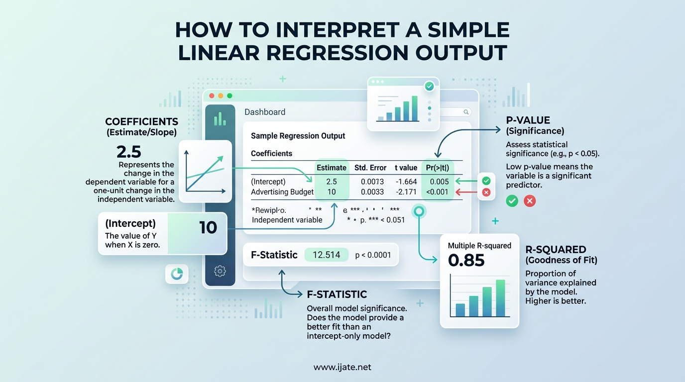
If you have ever run a regression in R, SPSS, Excel, or Python and stared at a wall of numbers wondering what any of it means, you are in the right place. Learning how to interpret a simple linear regression output is one of the most practical statistics skills you can build, because the same table format shows up across every major software tool.

I have spent years teaching students and analysts how to read these tables, and the good news is that every regression output follows the same basic structure. Once you understand what each number tells you, you can pick up any output from any tool and make sense of it in minutes.

This guide walks through every component of a simple linear regression output in plain language. No heavy formulas, no assumptions about your software, just clear explanations with a real worked example.

Here is the quick version of the interpretation process before we go deep:

1. Check the coefficients table for the slope and intercept estimates.
2. Look at the p-values to see if those coefficients are statistically significant.
3. Read R-squared to understand how well the model fits the data.
4. Examine the residual standard error to gauge prediction accuracy.
5. Review the F-statistic to test overall model significance.
6. Verify that the four regression assumptions are met using diagnostic plots.

Now let us break each of those steps down thoroughly.

What Is Simple Linear Regression?

Simple linear regression is a statistical method that models the straight-line relationship between two continuous variables. You have one independent variable (also called the predictor or explanatory variable) and one dependent variable (also called the response or outcome variable).

The goal is to fit the best possible straight line through your data points so you can use that line to predict the dependent variable from the independent variable. The method that finds this best-fitting line is called ordinary least squares, often abbreviated as OLS.

Least squares works by minimizing the sum of the squared vertical distances between each data point and the regression line. Think of those vertical distances as errors, also known as residuals. The smaller those errors are overall, the better the line fits your data.

For example, if you wanted to predict exam scores based on hours studied, simple linear regression would fit a line through a scatter plot of study hours versus scores. That line becomes your predictive model, and the regression output tells you everything about how reliable that model is.

The Regression Equation Explained

Every simple linear regression produces an equation that takes this form:

y = b0 + b1x

Here, y is the predicted value of the dependent variable. The variable x is the value of the independent variable you plug in. The term b0 is the intercept, which is the predicted value of y when x equals zero. The term b1 is the slope coefficient, which tells you how much y changes for every one-unit increase in x.

The intercept can be meaningful or meaningless depending on context. If x represents study hours and zero hours is a realistic scenario, the intercept is the predicted score for someone who did not study at all. But if x represents something like body weight, a value of zero might be impossible, making the intercept mathematically necessary but practically uninterpretable.

The slope coefficient is usually the number you care about most. If b1 equals 5.2 in the study hours example, that means each additional hour of studying is associated with a 5.2-point increase in exam score, on average.

A positive slope means the variables move in the same direction: as x increases, y increases. A negative slope means they move in opposite directions: as x increases, y decreases. The sign of the coefficient tells you the direction of the relationship at a glance.

How to Read the Coefficients Table

The coefficients table is the heart of any regression output, and it is also where most beginners get stuck. Once you decode the four or five columns in this table, you have conquered the hardest part of interpreting regression output.

Every coefficients table, whether it comes from R, SPSS, Excel, or Python, contains the same core columns. Let us walk through each one.

The Estimate Column

The Estimate column gives you the actual numbers for the intercept and slope. These are the b0 and b1 values that go into your regression equation. In R output, this column is labeled Estimate. In SPSS, it is labeled B. In Excel, it appears under Coefficients.

This is where you read off the practical effect size. A slope estimate of 5.2 tells you the magnitude of the effect: for every one-unit increase in your independent variable, your dependent variable changes by 5.2 units.

The Standard Error Column

The standard error tells you how precise that estimate is. Think of it as a measure of uncertainty around the coefficient. A smaller standard error means you can be more confident that the true slope is close to the estimated value. A larger standard error means the estimate is less reliable.

The standard error is not a number you interpret directly in most cases. Instead, it feeds into the t-statistic and confidence interval calculations. But understanding that a smaller standard error is better helps you make sense of the rest of the table.

The t-statistic Column

The t-statistic is calculated by dividing the estimate by its standard error. It tells you how many standard errors the estimate is away from zero. A t-value of 4.0, for example, means the estimate is four standard errors above zero.

As a rough rule of thumb, a t-statistic with an absolute value greater than 2 suggests the coefficient is statistically significant. Larger absolute t-values mean stronger evidence against the null hypothesis that the true coefficient is zero.

The p-value Column

The p-value is the probability of observing a coefficient at least as extreme as the one you got, assuming the null hypothesis is true. In regression, the null hypothesis for each coefficient is that the true value is zero, meaning the independent variable has no effect on the dependent variable.

The standard threshold for significance is a p-value less than 0.05. If your p-value is below 0.05, you reject the null hypothesis and conclude that the coefficient is statistically significant. If the p-value is above 0.05, you fail to reject the null hypothesis, meaning you do not have enough evidence to say the variable has a real effect.

One important nuance: a high p-value does not prove there is no relationship. It only means your sample does not provide strong enough evidence to conclude that a relationship exists. This distinction trips up a lot of people.

Significance Codes and Asterisks

In R output, you will see significance codes printed next to p-values as a series of asterisks. One asterisk means the p-value is between 0.01 and 0.05. Two asterisks means between 0.001 and 0.01. Three asterisks means below 0.001. A period means between 0.05 and 0.1, which is sometimes called marginally significant.

These codes are just shorthand so you can scan the table quickly. SPSS and Excel show the exact p-value instead, so you apply the same 0.05 threshold manually.

Confidence Intervals for Coefficients

Many outputs also include a 95 percent confidence interval for each coefficient. This interval gives you a range of plausible values for the true coefficient. For example, if the slope estimate is 5.2 with a confidence interval of 3.1 to 7.3, you can be 95 percent confident that the true slope falls somewhere in that range.

If the confidence interval does not include zero, the coefficient is statistically significant at the 0.05 level. This is another way to check significance without looking at p-values directly.

Interpreting R-squared and Adjusted R-squared

R-squared, also called the coefficient of determination, tells you what proportion of the variation in your dependent variable is explained by your independent variable. It ranges from 0 to 1, and you can also express it as a percentage.

An R-squared of 0.85 means that 85 percent of the variation in the dependent variable is accounted for by the independent variable through the regression line. The remaining 15 percent is unexplained variation, which comes from other factors or random noise.

People constantly ask what counts as a good R-squared value, and the honest answer is that it depends entirely on your field. In physics and engineering, you might expect R-squared values above 0.95 because physical systems are highly predictable. In social sciences and psychology, an R-squared of 0.30 might be perfectly respectable because human behavior has a lot of unmeasured variability.

Comparing R-squared to benchmarks from your own field is more meaningful than chasing an arbitrary universal threshold. A high R-squared in a weak study does not make the model good, and a moderate R-squared in a well-designed study can be valuable.

Adjusted R-squared vs R-squared

In simple linear regression with just one predictor, R-squared and adjusted R-squared will be nearly identical. The difference between them only becomes meaningful in multiple regression when you add more predictors to the model.

Regular R-squared always increases when you add more variables, even if those variables are useless. This creates a temptation to keep adding predictors to inflate the R-squared value. Adjusted R-squared penalizes you for adding variables that do not meaningfully improve the model.

In simple linear regression, you can focus on the regular R-squared. Just be aware that adjusted R-squared exists and becomes important the moment you move to multiple regression.

Residual Standard Error and Model Fit

The residual standard error, sometimes called the standard error of the estimate, tells you the average distance that the observed values fall from the regression line. It is measured in the same units as your dependent variable, which makes it directly interpretable.

If you are predicting exam scores on a 0 to 100 scale and your residual standard error is 7.5, that means your predictions are typically off by about 7.5 points in either direction. That is a very practical number for understanding prediction accuracy.

The residual standard error also connects to degrees of freedom, which equals your sample size minus the number of parameters estimated. In simple linear regression, you estimate two parameters (intercept and slope), so degrees of freedom equals n minus 2.

Smaller residual standard error values indicate tighter clustering of data points around the regression line, which means more precise predictions. Larger values mean the data points are more scattered and predictions carry more uncertainty.

Understanding the F-Statistic

The F-statistic tests the overall significance of your regression model. While the t-test on individual coefficients checks whether each predictor is significant on its own, the F-test asks whether the entire model does a better job of explaining the data than a model with no predictors at all.

The null hypothesis for the F-test is that all regression coefficients (except the intercept) equal zero. In other words, the model explains nothing.

In simple linear regression with only one predictor, the F-test and the t-test on the slope coefficient are testing the exact same thing. You will notice that the p-value for the F-statistic is identical to the p-value for the slope coefficient. Both tests answer the question: does this variable matter?

If the F-statistic p-value is below 0.05, your model is statistically significant overall. The F-test becomes more interesting in multiple regression, where it checks whether at least one of your several predictors is significant even if you cannot tell which one from the F-test alone.

A large F-statistic with a small p-value means your model captures a real relationship. A small F-statistic with a large p-value suggests the model is not meaningfully better than just using the mean of the dependent variable as your prediction.

A Complete Annotated Example: Reading Output Line by Line

Let us walk through a complete regression output using a realistic example. Suppose we collected data from 30 students, recording their study hours per week and their final exam scores. We ran a simple linear regression with exam score as the dependent variable and study hours as the independent variable.

Here is what the output would look like and how to interpret each piece.

Step 1: The Call and Residuals Section

The top of the output shows the model formula, confirming which variable predicts which. Below that, you see a summary of the residuals giving the minimum, first quartile, median, third quartile, and maximum values.

The residuals summary gives you a quick sense of how spread out the errors are. If the median is close to zero and the quartiles are roughly symmetric, that is a good initial sign. Large asymmetry between the quartiles can hint at skewness or outliers.

Step 2: The Coefficients Table

The coefficients table shows two rows: one for the intercept and one for the slope (study hours). For this example, suppose the intercept estimate is 42.3 with a p-value of 0.0001, and the slope estimate is 5.1 with a p-value of 0.00002.

The intercept of 42.3 means that a student who studies zero hours is predicted to score 42.3 on the exam. The slope of 5.1 means each additional hour of studying per week is associated with a 5.1-point increase in exam score.

Both p-values are well below 0.05, marked with three asterisks in R output, meaning both coefficients are highly significant. The standard error for the slope might be 1.1, giving a t-statistic of about 4.6, which confirms strong significance.

Step 3: Residual Standard Error

Suppose the residual standard error is 8.4 on 28 degrees of freedom. This tells us predictions are typically off by about 8.4 points. Given that exam scores range from 0 to 100, an error of about 8 points is moderate but could be useful depending on your purpose.

Step 4: R-squared

Suppose the multiple R-squared is 0.43 and adjusted R-squared is 0.41. This means study hours explain about 43 percent of the variation in exam scores. The remaining 57 percent comes from other factors like prior knowledge, sleep, test difficulty, and random variation.

For educational data, explaining 43 percent of variation with a single predictor is reasonable. You would not expect study hours alone to determine exam performance completely.

Step 5: F-statistic

Suppose the F-statistic is 21.3 with a p-value of 0.00009. This confirms the model is highly significant overall. The relationship between study hours and exam scores is not due to random chance.

Step 6: Putting It All Together

Here is how you would summarize this output in plain English: Study hours are a statistically significant predictor of exam scores (slope = 5.1, p less than 0.001). For each additional hour studied per week, exam scores increase by about 5.1 points. The model explains 43 percent of the variation in exam scores, with predictions typically accurate within about 8.4 points.

That summary is exactly what most reports, papers, and presentations need. You state the relationship, its significance, its magnitude, the model fit, and the prediction accuracy in a few sentences.

The Four Key Assumptions of Linear Regression

Interpreting the numbers in your regression output is only valid if the underlying assumptions of linear regression are met. If the assumptions are violated, your coefficients, p-values, and R-squared can all be misleading. Checking assumptions is not optional; it is part of doing regression properly.

Assumption 1: Linearity

The relationship between the independent and dependent variable must be linear. If the true relationship is curved or follows some other pattern, fitting a straight line will give you a misleading model.

You check linearity by creating a scatter plot of the two variables before running the regression. If the points roughly follow a straight-line pattern, the assumption is met. If you see a curve, a U-shape, or some other pattern, simple linear regression is not appropriate and you may need a transformation or a different model type.

Assumption 2: Independence of Residuals

The residuals must be independent of each other. This means one observation’s error should not predict another observation’s error. Violations commonly occur with time series data, where consecutive measurements are correlated, or with clustered data.

For cross-sectional data collected from independent individuals, this assumption is usually met by design. For time series or repeated measures, you may need specialized models like autoregressive models or mixed-effects models instead of simple linear regression.

Assumption 3: Homoscedasticity

Homoscedasticity means the spread of residuals should be roughly constant across all values of the independent variable. If the spread fans out or narrows as x increases, you have heteroscedasticity, which violates this assumption.

You check homoscedasticity with a residual plot, which puts fitted values on the x-axis and residuals on the y-axis. If the points form a random cloud with roughly equal width across the plot, the assumption is met. If you see a funnel shape where the spread increases or decreases, you have a problem.

When heteroscedasticity is present, your standard errors become unreliable, which means your t-statistics, p-values, and confidence intervals are no longer trustworthy. Common fixes include transforming the dependent variable or using robust standard errors.

Assumption 4: Normality of Residuals

The residuals should be approximately normally distributed, especially if you want to trust the p-values and confidence intervals. This assumption is about the residuals, not the variables themselves.

You check normality with a QQ plot, also called a quantile-quantile plot. If the points fall along a straight diagonal line, the residuals are approximately normal. Significant departures from the line indicate non-normality.

You can also use formal tests like the Shapiro-Wilk test or Kolmogorov-Smirnov test. However, these tests are sensitive to sample size: with very large samples they flag trivial deviations, and with very small samples they lack power. The QQ plot is usually more informative in practice.

What to Do When Assumptions Fail

If linearity fails, try a transformation like a log or square root of the dependent variable, or consider a polynomial or nonlinear model. If homoscedasticity fails, the same transformations often help, or you can use robust regression methods. If normality fails and your sample is reasonably large, the central limit theorem provides some protection, but severe departures may require bootstrapping or a different modeling approach.

Never skip the diagnostic checking step. Running a regression without checking assumptions is like building a house without inspecting the foundation. The structure might look fine on the surface, but it could collapse under scrutiny.

Common Mistakes When Interpreting Regression Output

Even when you understand each number in the output, certain conceptual mistakes can lead you to wrong conclusions. These errors come up constantly in student work, research papers, and business reports. Here are the most frequent ones I see.

Mistake 1: Confusing Correlation With Causation

A significant regression coefficient tells you that two variables are associated. It does not tell you that one causes the other. The classic example is ice cream sales and drowning deaths: both increase in summer, but ice cream does not cause drowning.

To establish causation, you need a controlled experiment, a strong theoretical basis, or advanced techniques like instrumental variables or difference-in-differences methods. Observational regression alone cannot prove causation, no matter how significant the p-value is.

Mistake 2: Treating a High R-squared as Proof of a Good Model

A high R-squared does not guarantee your model is correct. You can achieve a high R-squared with a model that violates assumptions, contains spurious correlations, or simply overfits the data. Always check assumptions and think about whether the relationship makes theoretical sense.

Conversely, a low R-squared does not mean your model is useless. In fields with inherently noisy data, a model that explains 20 percent of the variation can still provide valuable insights and useful predictions.

Mistake 3: Misinterpreting p-values

A p-value below 0.05 does not mean there is a 95 percent chance your hypothesis is true. It means that if the null hypothesis were true, there is only a 5 percent chance of seeing results this extreme. These are very different statements.

Also, a p-value of 0.051 versus 0.049 is practically meaningless as a difference, even though one is typically called significant and the other is not. Do not treat the 0.05 threshold as a magical cliff edge.

Mistake 4: Extrapolating Beyond the Data Range

Your regression model is only valid within the range of x values you observed. If your study hours data ranges from 1 to 20 hours per week, predicting a score for someone studying 50 hours is extrapolation, and the prediction could be wildly wrong.

The linear relationship might not hold outside the observed range. The student studying 50 hours might hit diminishing returns, or might be so overworked that their score actually drops. The straight-line model cannot capture these patterns.

Mistake 5: Ignoring the Intercept

People often focus entirely on the slope and ignore the intercept. But if the intercept is meaningless because x cannot realistically equal zero, your regression equation still contains that intercept, and predictions near the lower end of your x range can be affected by it.

Centering your independent variable by subtracting the mean can make the intercept interpretable. After centering, the intercept represents the predicted y value at the average x value, which is usually meaningful.

How to Report Regression Results in a Paper or Report

One of the biggest gaps in most regression guides is explaining how to communicate your findings. Whether you are writing a research paper, a business report, or a thesis, there are standard conventions for reporting regression results clearly.

The APA style, widely used in social sciences, recommends reporting the slope coefficient, standard error, t-statistic, p-value, and R-squared in a concise format. Here is an example sentence following APA conventions:

Study hours significantly predicted exam scores, b = 5.1, SE = 1.1, t(28) = 4.64, p less than .001. The model explained a significant proportion of variance in exam scores, R-squared = .43, F(1, 28) = 21.56, p less than .001.

That single pair of sentences communicates the slope, its precision, its significance, the model fit, and the overall model test. For a more detailed report, you would add the 95 percent confidence interval for the slope and a brief plain-language interpretation of what the coefficient means in context.

For business audiences, focus on practical significance rather than statistical jargon. Instead of citing p-values, describe the effect size in dollar or percentage terms. Instead of reporting R-squared, explain what proportion of the outcome the model accounts for in plain language.

Always include a scatter plot with the regression line when presenting results visually. This gives readers an immediate sense of the relationship strength, the spread of the data, and whether any outliers might be influencing the results.

Frequently Asked Questions

Conclusion

Learning how to interpret a simple linear regression output comes down to understanding six core components: the regression equation, the coefficients table, R-squared, residual standard error, the F-statistic, and the diagnostic checks for assumptions. Each piece tells you something different, and together they give you a complete picture of your model.

Start with the coefficients to understand the direction and magnitude of the relationship. Check the p-values and confidence intervals to assess significance. Read R-squared to see how well the model fits. Examine the residual standard error for prediction accuracy. Review the F-statistic for overall model significance. And always verify that the four assumptions of linearity, independence, homoscedasticity, and normality are reasonably met.

The next step is to practice. Take a dataset, run a simple regression in whatever software you have available, and work through each component of the output using this guide. The more tables you read, the faster and more confident you will become. Regression output stops being intimidating once you know exactly where to look and what each number means.