How to Interpret Bayesian Results in JASP (2026 Guide)

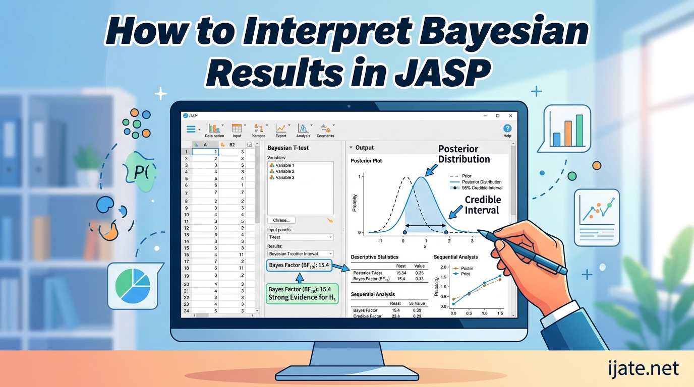
Bayesian statistics can feel intimidating the first time you stare at a JASP output table. I remember my own confusion: numbers everywhere, models I did not ask for, and a “Bayes factor” that seemed to defy explanation. If you are in that spot right now, this guide is for you.

We are going to walk through how to interpret Bayesian results in JASP, one component at a time, using plain language and real examples. By the end, you will know exactly what BF₁₀ means, how to read a posterior summary table, and how to report your findings with confidence.

JASP has become one of the most popular open-source tools for Bayesian analysis because it pairs a clean graphical interface with rigorous statistical engines. Researchers, students, and data scientists use it daily to run Bayesian t-tests, ANOVAs, regressions, and more. But the software gives you a lot of output, and that output uses terminology that differs from the frequentist statistics most of us learned first.

This guide covers the core building blocks you need: Bayes factors, posterior distributions, credible intervals, model comparison tables, and reporting standards. We will also address the questions that surface repeatedly on forums like r/statistics and the JASP community board.

Understanding Bayesian Analysis Basics

Bayesian analysis interprets probability as a measure of believability or confidence in a hypothesis, rather than as a long-run frequency. In practice, this means you can make direct probability statements about your parameters and hypotheses. That single shift changes how you read every output table JASP produces.

Three concepts form the backbone of every Bayesian analysis: the prior, the likelihood, and the posterior. The prior distribution encodes what you believed before seeing data. The likelihood captures how plausible the observed data are under different parameter values. The posterior distribution combines the two and represents your updated belief after the data have been incorporated.

JASP handles all of this under the hood. You choose a test, optionally adjust a prior width setting, and the software computes the posterior and the Bayes factor. Your job is to interpret what comes out.

Why Use JASP for Bayesian Analysis?

JASP is open-source, academically validated, and designed to make Bayesian methods accessible without writing code. It defaults to sensible prior choices (typically the Cauchy distribution centered at zero, known as the JZS prior) so you can run a Bayesian t-test or ANOVA without needing to specify a custom prior.

The software also shows both Bayesian and frequentist results side by side. This side-by-side layout makes it easier to compare approaches and helps you spot when the two frameworks agree or disagree.

Forum users on r/statistics consistently report that JASP’s graphical interface reduces coding errors compared to writing R scripts manually. The community forum at forum.cogsci.nl provides peer support, and results from JASP align with established R packages like BayesFactor.

Bayesian vs Frequentist: A Quick Contrast

The most common confusion I see is conflating p-values with Bayes factors. They answer different questions. A p-value tells you the probability of observing data as extreme as yours, assuming the null hypothesis is true. A Bayes factor tells you how much more likely your data are under one hypothesis compared to another.

That distinction matters. A p-value cannot tell you the probability that your hypothesis is true. A Bayes factor, combined with prior odds, gives you a posterior odds ratio that directly quantifies the relative support for competing models.

Here is a quick comparison to keep handy:

• Frequentist p-value: Probability of data given the null hypothesis is true.
• Bayes factor: Relative evidence for one model versus another, based on the data.
• Posterior probability: Updated probability of a hypothesis after seeing the data.
• Credible interval: The range that contains the parameter with a specified probability.

How to Interpret Bayesian Results in JASP: Core Components

Every Bayesian analysis in JASP produces a handful of core outputs regardless of which test you run. Once you understand these components, you can interpret any Bayesian result the software generates. Let me break them down one by one.

The Bayes Factor (BF₁₀ and BF₀₁)

The Bayes factor is the single most important number in any JASP Bayesian output. It quantifies the evidence that your data provide for one hypothesis relative to another. JASP reports it as either BF₁₀ (evidence for the alternative hypothesis versus the null) or BF₀₁ (evidence for the null versus the alternative).

BF₁₀ and BF₀₁ are reciprocals of each other. If BF₁₀ equals 5, then BF₀₁ equals 0.2. JASP lets you toggle between the two, which can be disorienting at first. My advice: pick a convention and stick with it. I default to BF₁₀ because a value above 1 means support for the alternative, which aligns with how most researchers frame hypotheses.

A Bayes factor of BF₁₀ = 3 means the observed data are three times more likely under the alternative hypothesis than under the null. A BF₁₀ of 0.33 means the data are three times more likely under the null. The number itself is a ratio of marginal likelihoods, but you do not need to compute it manually. JASP does the heavy lifting.

Posterior Distributions and Posterior Summaries

While the Bayes factor tells you which hypothesis the data support, the posterior distribution tells you what the parameter values likely are. JASP provides a posterior summary table that lists the posterior mean, standard deviation, and credible interval for each parameter.

The posterior mean is your best single estimate of the parameter after combining your prior with the data. The credible interval gives you a range of plausible values. Unlike a confidence interval, a 95% credible interval has a direct interpretation: there is a 95% probability that the parameter falls within this range, given the data and the model.

JASP also plots the posterior distribution when you select the appropriate option. These plots are gold for interpretation. A posterior distribution tightly centered around a single value means high precision. A wide, flat posterior means substantial uncertainty remains.

Credible Intervals Explained

I want to highlight credible intervals separately because they are the source of so much confusion. A 95% credible interval in Bayesian analysis means there is a 95% probability that the true parameter value lies within the interval, given everything you know (the data plus the prior).

This is a fundamentally different statement from a 95% confidence interval, which technically means that if you repeated the experiment infinitely many times, 95% of the computed intervals would contain the true parameter. The confidence interval says nothing about the probability that the parameter lies in this specific interval.

In JASP output, you will typically see credible intervals labeled as “95% Credible Interval” in the posterior summary table. Some analyses allow you to adjust this to 90% or 99%. For most academic reporting, 95% is the standard.

Model Comparison Tables

One of the most common questions on the JASP forum is: “Why does JASP show so many models?” This happens because Bayesian analysis compares multiple models, not just one null and one alternative. In a Bayesian regression with three predictors, for example, JASP evaluates every possible combination of those predictors.

For each model, JASP reports the prior model probability, the posterior model probability, and a Bayes factor comparing that model to the null model. The model with the highest posterior probability has the most support from the data.

This multi-model approach is actually one of the strengths of Bayesian analysis in JASP. Instead of forcing you to commit to a single model, it accounts for uncertainty across all plausible models. The result is a more honest picture of what your data do and do not support.

Inclusion Bayes Factors

When JASP compares many models, you also get an “analysis of effects” table that reports inclusion Bayes factors. An inclusion BF quantifies the evidence for including a specific predictor across all models, averaged by model probability. Think of it as the overall evidence that a particular variable matters.

An inclusion BF of 12 for a predictor means the data are 12 times more likely under models that include that predictor than under models that exclude it. This model-averaged approach is more robust than looking at a single model because it does not pretend you knew the correct model in advance.

Forum users on r/bayesian consistently note that model averaging provides more robust estimates than single model selection. I have found this especially true in exploratory analyses where theory does not dictate a specific model in advance.

Interpreting Bayes Factors: Thresholds and Meaning

The Bayes factor interpretation scale is the most frequently requested reference on statistics forums. JASP uses the classification scheme popularized by Jeffreys (1961) and refined by Lee and Wagenmakers (2013). Here is the breakdown that JASP applies automatically in its output annotations.

Bayes Factor Interpretation Scale

JASP labels Bayes factors with qualitative descriptors so you do not have to memorize thresholds. Still, knowing the scale helps you communicate results clearly. The thresholds apply to BF₁₀ (evidence for the alternative); invert them for BF₀₁.

• BF = 1: No evidence. The data support neither hypothesis over the other.
• BF between 1 and 3: Anecdotal evidence for the alternative.
• BF between 3 and 10: Moderate evidence for the alternative.
• BF between 10 and 30: Strong evidence for the alternative.
• BF between 30 and 100: Very strong evidence for the alternative.
• BF above 100: Decisive (extreme) evidence for the alternative.

For BF₀₁, the same thresholds apply in reverse. A BF₀₁ of 5 means moderate evidence for the null hypothesis. A BF₀₁ below 0.3 (equivalent to BF₁₀ above 3.33) indicates moderate or stronger evidence for the alternative, which matches what users on r/AskStatistics frequently report.

What Does a Bayes Factor of 1 Mean?

A Bayes factor of exactly 1 means the data are equally likely under both hypotheses. The evidence does not favor either side. This is the Bayesian equivalent of saying “I have no reason, based on this data, to prefer one hypothesis over the other.”

This is genuinely informative. Unlike a non-significant p-value, which leaves you in an ambiguous state, a BF near 1 tells you the data are insensitive. You can then decide whether to collect more data or conclude that no meaningful effect exists.

What Does a High Bayes Factor Mean?

A high Bayes factor (typically above 10) means the data strongly support the alternative hypothesis over the null. The higher the value, the more decisive the evidence. A BF₁₀ of 50 means the data are 50 times more likely under the alternative than under the null.

However, a high Bayes factor does not tell you the effect is large. It tells you the evidence is strong. The effect size comes from the posterior distribution and the credible interval, not from the Bayes factor itself. I have seen students conflate these two and report that a “large Bayes factor means a large effect.” It does not.

BF₁₀ vs BF₀₁: Which Should You Use?

This question comes up constantly. The answer is: use whichever framing makes your narrative clearer. If your finding supports the alternative hypothesis, report BF₁₀. If your finding supports the null, report BF₀₁ so the number is greater than 1 and easier to interpret on the standard scale.

For example, if BF₁₀ = 0.2, you could report “BF₁₀ = 0.2, indicating support for the null” or equivalently “BF₀₁ = 5, indicating moderate evidence for the null.” The second phrasing is cleaner because 5 maps directly onto the interpretation scale.

Common Bayes Factor Mistakes

I see a handful of recurring mistakes when people interpret Bayes factors in JASP. Here are the ones to avoid:

• Treating BF as a probability: A Bayes factor is a ratio of likelihoods, not a probability. BF = 10 does not mean a 90% probability that the alternative is true.
• Ignoring the prior: The Bayes factor depends on the prior you specify. A wider prior can reduce the BF for the same data.
• Comparing BFs across different studies: Bayes factors are specific to the models and priors used. Cross-study comparisons require identical setups.
• Confusing absence of evidence with evidence of absence: A BF near 1 means the data are inconclusive, not that the null is true.

Step-by-Step Guide: Reading JASP Output Tables

Now let us walk through the actual output tables you will see in JASP for the most common analyses. I will cover the model comparison table, posterior summary table, and the specific outputs for ANOVA, regression, and t-tests.

Reading the Model Comparison Table

The model comparison table appears in Bayesian regression, ANOVA, and other multi-model analyses. Each row represents a different model (a different combination of predictors or effects). Here is how to read it, column by column:

• Models: Lists which predictors or effects each model includes.
• P(M): Prior model probability. By default, JASP assigns equal probability to all models.
• P(M|data): Posterior model probability. This is the probability of each model after seeing the data. Higher is better.
• BF_M: Bayes factor comparing each model to the null model.
• Error %: A numerical stability metric. Values below 1% are generally fine. If you see high error percentages, increase the number of samples.

The model with the highest P(M|data) has the most support from the data. But do not stop there. Look at the spread of posterior probabilities across models. If one model dominates with P(M|data) above 0.9, you have strong evidence for that specific model. If probabilities are spread thinly across several models, no single model stands out.

Reading the Posterior Summary Table

The posterior summary table appears below or alongside the model comparison table. It provides parameter estimates for each predictor. Here is what each column means:

• Coefficient: The name of the predictor or intercept.
• Mean: The posterior mean, which is your best estimate of the parameter value.
• SD: The posterior standard deviation, representing uncertainty.
• 95% Credible Interval: The range within which the parameter falls with 95% probability.

If the 95% credible interval for a coefficient does not include zero, that is evidence the predictor has a meaningful effect. The posterior mean tells you the direction and magnitude of that effect.

JASP can also display the marginal posterior distribution for each coefficient as a plot. These plots show the full shape of the posterior, not just summary statistics. A posterior that is sharply peaked indicates a precise estimate. A posterior that is wide or bimodal indicates uncertainty or model instability.

Interpreting Bayesian ANOVA Output

In a Bayesian ANOVA, the model comparison table lists models corresponding to different combinations of main effects and interactions. The analysis of effects table below it reports inclusion Bayes factors for each factor, averaged across all models.

Read the inclusion BF for each effect first. An inclusion BF above 3 means moderate evidence that the effect matters. An inclusion BF below 0.33 means moderate evidence that the effect does not matter. Values between 0.33 and 3 are inconclusive.

For post-hoc comparisons and parameter estimates, look at the posterior summary and the descriptive plots JASP generates. These give you the same credible interval and posterior mean information as in regression, but broken down by factor levels.

Interpreting Bayesian Regression Output

Bayesian linear regression in JASP produces the model comparison table and posterior summary table described above. Start with the model comparison table to see which combination of predictors has the most support. Then check the analysis of effects table for inclusion Bayes factors on each predictor.

For the posterior summary, focus on the mean and credible interval for each coefficient. If you selected “model averaging” (the default), the posterior estimates are weighted across all models by their posterior probabilities. This gives you more stable estimates than relying on a single best model.

The JASP case study on Bayesian linear regression recommends reporting both the best-supported model and the model-averaged estimates. This gives readers the full picture: which model fits best, and what the parameter estimates look like when you account for model uncertainty.

Interpreting Bayesian T-Test Output

The Bayesian t-test is the simplest Bayesian output in JASP. You get a single Bayes factor (BF₁₀) comparing the alternative hypothesis (there is a difference between groups) to the null (no difference). JASP reports this alongside the frequentist t-test result.

The descriptive plot shows the posterior distribution for the effect size (delta). Check whether the 95% credible interval for delta includes zero. If it does not, the effect is credibly different from zero. Combine this with the Bayes factor: a BF₁₀ above 10 with a credible interval excluding zero gives you strong, consistent evidence for a real effect.

JASP also offers a sequential analysis plot for t-tests, which shows how the Bayes factor changes as data accumulate. This is useful for understanding whether more data would strengthen or weaken your conclusion.

Credible Intervals vs Confidence Intervals

This distinction deserves its own section because it is the single most misunderstood concept for people transitioning from frequentist to Bayesian analysis. I have seen experienced researchers mix these up in published papers.

The Fundamental Difference

A 95% credible interval means there is a 95% probability that the parameter lies within the interval, given the observed data and the model. You can make direct probability statements about the parameter. This is the interpretation most people intuitively want from a confidence interval but never get.

A 95% confidence interval means that if you repeated the study many times, 95% of the intervals you computed would contain the true parameter. You cannot say there is a 95% probability that this specific interval contains the parameter. The parameter is fixed; the interval is random.

Practical Interpretation in JASP

In JASP, credible intervals appear in the posterior summary table for every Bayesian analysis. When you report them, you can say: “The posterior mean for the effect was 0.45, with a 95% credible interval of [0.12, 0.78].” Readers familiar with Bayesian methods will understand this directly.

If your audience is primarily familiar with frequentist methods, add a brief note explaining that credible intervals allow direct probability interpretation. This avoids confusion and positions your results correctly within the Bayesian framework.

How to Report Credible Intervals

Report the posterior mean and the credible interval together. State the credible level (95% is standard). If the interval excludes zero for a parameter of interest, note that the effect is credibly different from zero. Avoid the phrase “statistically significant” when reporting Bayesian results; instead, describe the strength of evidence using the Bayes factor and the precision of the estimate using the credible interval.

Practical Tips and Common Pitfalls

Over years of running Bayesian analyses in JASP, I have collected a set of practical tips that go beyond the basics. These address the questions and confusions that come up most often on forums and in consulting sessions.

Setting Your Prior Width

JASP defaults to a Cauchy prior width of 0.707 (the “medium” JZS prior) for t-tests and similar defaults for other analyses. This default works well for most social science research where effect sizes tend to be small to moderate. For fields with typically large effects (some areas of psychology, sensory studies), you may want to narrow the prior.

The prior width affects your Bayes factor. A wider prior spreads probability across a larger range of effect sizes, which can reduce the BF when the true effect is small. JASP lets you run a robustness check that varies the prior width and shows how the BF changes. Always run this check if your BF is near a threshold like 3 or 10.

Sequential Analysis

JASP offers sequential analysis plots for several Bayesian tests. These plots show how the Bayes factor evolves as you add more data points, one at a time. This is one of the genuine advantages of Bayesian methods: you can monitor evidence as it accumulates without penalty.

If your sequential plot shows the BF climbing steadily toward strong evidence, you can be confident in your conclusion. If the BF bounces around or oscillates near 1, the evidence is unstable and you may need more data. This diagnostic is far more informative than a single static p-value.

Robustness Checking

Always check the robustness of your Bayes factor to prior specification. JASP provides a “Bayes factor robustness check” plot that varies the prior width (r scale) from very narrow to very wide and shows how the BF responds. If your BF stays above your evidence threshold across a wide range of prior widths, your conclusion is robust. If the BF crosses below 3 or 10 when you change the prior, report that sensitivity honestly.

Reporting Guidelines for Academic Papers

The JASP guidelines for conducting and reporting a Bayesian analysis (published in PMC, with over 1300 citations) recommend including the following in any report:

• The Bayes factor and which hypotheses it compares (e.g., BF₁₀ = 7.5).
• The prior specification, including prior width if non-default.
• The posterior mean and 95% credible interval for key parameters.
• A robustness check if the result depends on prior choice.
• An effect size estimate with credible interval.
• Software version (JASP version number) for reproducibility.

Following these guidelines makes your results transparent and reproducible. Reviewers familiar with Bayesian methods will look for this information, and including it proactively strengthens your submission.

When to Use Bayesian Instead of Frequentist

You do not need to abandon frequentist methods entirely. Bayesian analysis shines when you want to: quantify evidence for the null hypothesis, monitor evidence as data accumulate, incorporate prior knowledge, or make direct probability statements about parameters. If none of these apply, frequentist methods remain perfectly serviceable.

Many researchers run both and report both. JASP makes this trivial since it displays both outputs side by side. When the two agree, your conclusion is on solid ground. When they disagree, the Bayesian result is often more informative because it can distinguish between “evidence for no effect” and “insufficient evidence either way.”

FAQ’s

Conclusion

Learning how to interpret Bayesian results in JASP opens up a more informative and intuitive way to analyze data. The Bayes factor gives you a continuous measure of evidence that can support the null just as well as the alternative. The posterior distribution shows you the full range of plausible parameter values, and credible intervals let you make direct probability statements that match how you actually think about your results.

Start with the Bayes factor to gauge evidence strength. Move to the posterior summary for parameter estimates. Use credible intervals to communicate precision. Run a robustness check when your BF sits near a decision threshold. And follow the JASP reporting guidelines so your results are transparent and reproducible.

The more you practice reading these outputs, the more natural they become. Open JASP, load a sample dataset, run a Bayesian t-test, and walk through each table using this guide. Within a few sessions, interpreting Bayesian results will feel as routine as reading a p-value once did, only far more informative.