How to Run a One-Way ANOVA in SPSS (2026 Guide)

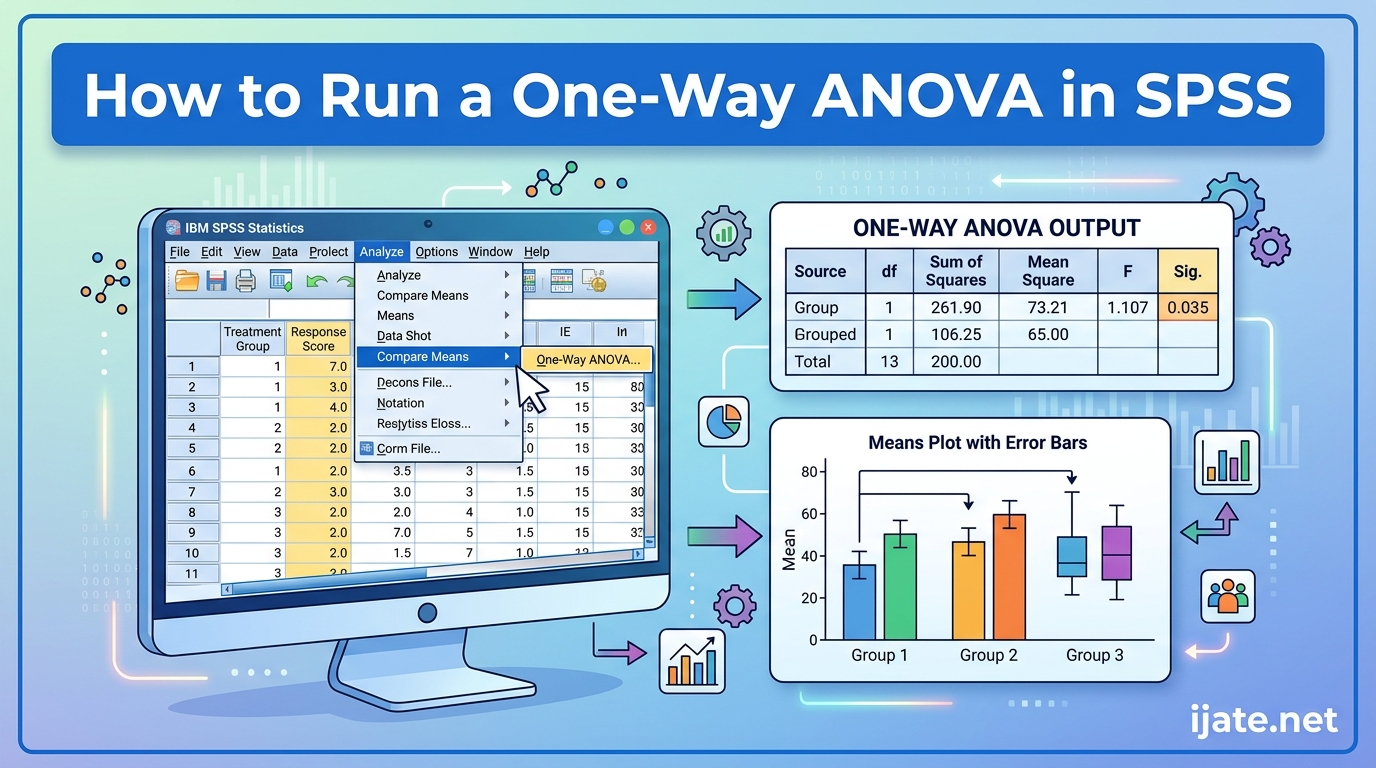
Learning how to run a one-way ANOVA in SPSS opens the door to comparing three or more group means in a single analysis. To run a one-way ANOVA in SPSS, click Analyze > Compare Means > One-Way ANOVA, move your continuous dependent variable to the Dependent List box, move your categorical independent variable to the Factor box, select Post Hoc tests and Options, then click OK. That menu path is the core procedure, and the rest of this guide walks you through every dialog, assumption, output table, and reporting step in detail.

A one-way ANOVA, also called one-way analysis of variance, is a parametric test that determines whether the means of two or more independent groups differ significantly. The test produces an F-statistic and a p-value that tell you whether at least one group mean differs from the others. You can see a real-world application of ANOVA in educational research to understand how this test is used in published studies.

In this guide, our team covers everything from data setup and assumption checking to output interpretation, APA reporting, and troubleshooting errors that trip up SPSS users. Whether you are a student running your first analysis or a researcher refreshing your skills, this walkthrough gives you the full procedure for 2026.

Quick Steps: How to Run a One-Way ANOVA in SPSS

Here is the fast version of how to run a one-way ANOVA in SPSS. Each step below corresponds to a section later in this guide where I explain the details.

1. Open your dataset in SPSS and confirm your dependent variable is continuous (Scale) and your independent variable is categorical (Nominal or Ordinal).
2. Click Analyze > Compare Means > One-Way ANOVA to open the main dialog box.
3. Move your dependent variable to the Dependent List box using the blue arrow.
4. Move your independent variable (the grouping variable) to the Factor box.
5. Click Post Hoc, select Tukey HSD (for equal variances) or Games-Howell (for unequal variances), then click Continue.
6. Click Options, check Descriptive Statistics, Homogeneity of Variance Test, and Means Plot, then click Continue.
7. Click OK to run the analysis and generate the output in the SPSS Output Viewer.

That seven-step sequence is what most SPSS users follow for a standard one-way ANOVA. The sections below expand on each step, including how to set up your data, which assumptions to check, and how to interpret every output table.

What Is a One-Way ANOVA?

A one-way ANOVA is a statistical procedure that compares the means of three or more independent groups to test whether at least one group mean differs from the rest. The term “one-way” means the analysis includes a single independent variable, also called a factor, with two or more levels. SPSS uses the term “factor” to describe this categorical grouping variable in its One-Way ANOVA dialog.

The test works by partitioning the total variance in your data into two components. Between-groups variance reflects differences among group means, while within-groups variance reflects individual differences inside each group. SPSS divides the between-groups mean square by the within-groups mean square to produce the F-statistic, and the associated p-value tells you whether the observed F is large enough to reject the null hypothesis.

A significant F-statistic (typically p less than 0.05) tells you that at least one group differs from another, but it does not tell you which groups differ. That is why post hoc tests like Tukey HSD are essential after a significant ANOVA result. You can see how ANOVA is applied in educational research to observe this process in published work.

Many students confuse the one-way ANOVA with an independent t-test. The key difference is scope: a t-test compares exactly two groups, while a one-way ANOVA handles three or more groups in a single omnibus test. Running multiple t-tests instead of one ANOVA inflates your Type I error rate, which is why ANOVA is the preferred approach when you have more than two groups.

Assumptions and Data Requirements for One-Way ANOVA

One-way ANOVA is a parametric test, which means it relies on specific statistical assumptions about your data. Checking these assumptions before running the test is critical because violations can lead to inaccurate results and misleading conclusions.

Assumption 1: Continuous Dependent Variable

Your dependent variable must be measured at the interval or ratio level. In SPSS, this means the variable should be set to Scale measurement type. Examples include test scores, reaction times, weights, and revenue figures. If your dependent variable is categorical, one-way ANOVA is not appropriate and you should consider chi-square tests instead.

Assumption 2: Categorical Independent Variable with Two or More Groups

Your independent variable, the factor, must be categorical with at least two levels. In practice, most one-way ANOVAs involve three or more groups because two groups can be compared with a t-test. Examples of factors include treatment condition, education level, or region. SPSS requires this variable to be coded as Nominal or Ordinal.

Assumption 3: Independence of Observations

Each observation in your dataset must be independent of all other observations. This means no participant appears in more than one group, and there is no pairing or clustering in the design. Violations of independence are serious because they cannot be corrected statistically. If your design involves repeated measures on the same participants, use a repeated measures ANOVA instead.

Assumption 4: No Significant Outliers

Outliers can distort group means and inflate the within-groups variance, reducing the power of your ANOVA. Before running the test, examine your data with boxplots (Graphs > Chart Builder > Boxplot) or explore cases using Analyze > Descriptive Statistics > Explore. Remove or transform outliers only if you have a sound statistical or methodological justification.

Assumption 5: Normality of the Dependent Variable in Each Group

The dependent variable should be approximately normally distributed within each group. For sample sizes above 30 per group, the ANOVA F-test is robust to moderate normality violations thanks to the Central Limit Theorem. For smaller samples, check normality with the Shapiro-Wilk test (Analyze > Descriptive Statistics > Explore > Plots > Normality plots with tests) or inspect Q-Q plots.

If normality is violated with small samples, consider a nonparametric alternative like the Kruskal-Wallis test (Analyze > Nonparametric Tests > Independent Samples). The Kruskal-Wallis test does not assume normality and works with ranked data, making it suitable for ordinal dependent variables as well.

Assumption 6: Homogeneity of Variances

The variance of the dependent variable should be roughly equal across all groups. SPSS tests this assumption automatically when you check “Homogeneity of variance test” in the Options dialog. The output produces Levene’s test, where a non-significant result (p greater than 0.05) means variances are approximately equal and the standard ANOVA is appropriate.

If Levene’s test is significant, meaning variances are unequal, you should use the Welch ANOVA instead of the standard one-way ANOVA. SPSS does not produce the Welch test from the One-Way ANOVA dialog directly, but you can access it through Analyze > Compare Means > One-Way ANOVA > Options > Welch, or by using the General Linear Model > Univariate dialog where Brown-Forsythe and Welch adjustments are available.

Data Setup in SPSS Before Running One-Way ANOVA

Proper data setup prevents most errors that SPSS users encounter when running one-way ANOVA. Your data should be in a single file where each row represents one participant or case and each column represents one variable.

Setting Up Your Variables

In Variable View, define two key variables. The first is your dependent variable, which must be set to Scale measurement type and should contain numeric values. The second is your independent variable (the grouping variable), which should be set to Nominal or Ordinal measurement type and contain numeric group codes.

For example, if you are comparing exam scores across three teaching methods, your dependent variable might be “Score” and your independent variable might be “Method” coded as 1, 2, and 3 for the three teaching approaches. Use the Values column in Variable View to add labels (e.g., 1 = Lecture, 2 = Online, 3 = Hybrid) so SPSS displays meaningful group names in the output.

Converting String Variables to Numeric Codes

A common pain point on the r/spss community is that SPSS will not accept string variables in the Factor box. If your grouping variable is currently a string (for example, text values like “Beginner,” “Intermediate,” “Advanced”), you need to convert it to numeric codes before running the ANOVA.

To convert a string variable, go to Transform > Automatic Recode. Select your string variable, give the new variable a name, and click OK. SPSS automatically assigns sequential numeric codes (1, 2, 3) to each unique string value and preserves the original text as value labels. This recoded variable can then be placed in the Factor box.

Handling Missing Data

Missing values can affect your ANOVA results. SPSS uses listwise deletion by default in the One-Way ANOVA procedure, meaning any case with a missing value on either the dependent or independent variable is excluded from the analysis. Check your missing data patterns with Analyze > Descriptive Statistics > Frequencies before running the test.

If you have substantial missing data, consider whether the missingness is random or systematic. For random missing data, listwise deletion is generally acceptable. For larger amounts of missing data, consider multiple imputation (Analyze > Multiple Imputation) before running the ANOVA to preserve statistical power.

How to Run a One-Way ANOVA in SPSS: Step by Step

Now I will walk through the complete procedure for how to run a one-way ANOVA in SPSS, covering every dialog box in the order you will encounter them.

Step 1: Open the One-Way ANOVA Dialog

From the SPSS menu bar, click Analyze > Compare Means > One-Way ANOVA. The One-Way ANOVA dialog box appears with a list of your variables on the left and three main boxes on the right: Dependent List, Factor, and a layer for covariates (which are not used in basic one-way ANOVA).

Step 2: Move Your Dependent Variable

Select your continuous dependent variable from the list on the left. Click the blue arrow next to the Dependent List box to move it over. You can include multiple dependent variables if you want to run separate ANOVAs on each, but the standard approach uses one dependent variable at a time.

Step 3: Move Your Independent Variable to the Factor Box

Select your categorical grouping variable and click the blue arrow next to the Factor box to move it. SPSS requires this variable to be numeric (Nominal or Ordinal measurement type). If the variable is a string, you will see an error or the variable will not appear in the list at all.

Step 4: Configure Post Hoc Tests

Click the Post Hoc button to open the Post Hoc Multiple Comparisons dialog. This dialog is where you choose which post hoc tests to run after the omnibus F-test. SPSS divides the available tests into two groups based on whether equal variances are assumed.

If you expect equal variances (which you will confirm with Levene’s test in the output), select Tukey HSD. Tukey is the most widely used post hoc test because it controls the family-wise error rate well and is easy to interpret. Other options for equal variances include Bonferroni (more conservative), Scheffe (best for unequal group sizes), and Dunnett (used when comparing multiple groups against a single control group).

If you expect unequal variances, select Games-Howell from the “Equal Variances Not Assumed” section. Games-Howell is the recommended alternative when Levene’s test is significant because it adjusts for both unequal variances and unequal sample sizes. After selecting your tests, click Continue.

Step 5: Configure Options

Click the Options button to open the Options dialog. Here you select which additional statistics and tests SPSS should produce alongside the main ANOVA table. Check the following items:

• Descriptive Statistics: Produces group means, standard deviations, standard errors, 95 percent confidence intervals, and minimum and maximum values for each group.
• Homogeneity of Variance Test: Runs Levene’s test, which checks whether group variances are approximately equal. This output is essential for deciding whether to trust the standard ANOVA or switch to the Welch alternative.
• Means Plot: Produces a simple line chart showing group means, which gives you a quick visual sense of differences between groups.
• Brown-Forsythe and Welch (if available in your SPSS version): These are robust alternatives that adjust for unequal variances.

After checking these options, click Continue to return to the main dialog.

Step 6: Run the Analysis

Click OK to run the one-way ANOVA. SPSS processes the analysis and sends all results to the Output Viewer. The output typically includes the Descriptives table, the Test of Homogeneity of Variances table, the ANOVA table, and any Post Hoc tables you selected. The next section explains how to read each of these.

Step 7 (Optional): Configure Contrasts

The Contrasts button in the One-Way ANOVA dialog lets you test specific hypotheses about group differences rather than running all pairwise comparisons. For example, you can set up a polynomial contrast to test for linear or quadratic trends across ordered groups, or you can define custom contrasts to compare specific combinations of group means. Most users do not need contrasts for a basic analysis, but they are useful when you have a priori hypotheses about specific group relationships.

SPSS Output Interpretation: Reading the ANOVA Results

Interpreting the SPSS output correctly is just as important as running the analysis itself. The Output Viewer displays several tables, and each one answers a different question about your data. Let me walk through them in the order they appear.

The Descriptives Table

The Descriptives table appears first and provides summary statistics for each group. For every level of your independent variable, you will see the group mean, standard deviation, standard error, 95 percent confidence interval for the mean, and the minimum and maximum values. The bottom row labeled “Total” shows the overall statistics across all groups combined.

Pay close attention to the group means and confidence intervals. If the confidence intervals for two groups do not overlap, those groups are likely significantly different. However, non-overlapping intervals are a rough guide, not a definitive test. The actual significance testing happens in the post hoc comparisons table.

The standard deviations across groups give you an early read on the homogeneity of variances assumption. If one group has a standard deviation two or three times larger than another, you may be heading toward a significant Levene’s test and will need to use the Welch alternative or Games-Howell post hoc test.

The Test of Homogeneity of Variances (Levene’s Test)

This table reports Levene’s statistic, the degrees of freedom (df1 and df2), and the significance value. The interpretation rule is straightforward: if the Sig. value is greater than 0.05, variances are approximately equal and the standard ANOVA is valid. If the Sig. value is less than 0.05, variances are significantly different, and you should rely on the Welch or Brown-Forsythe results instead.

A significant Levene’s test is one of the most common sources of confusion in the r/spss and r/statistics communities. Users frequently ask what to do when this test fails. The answer is to report the Welch ANOVA results rather than the standard F-test, and to use Games-Howell instead of Tukey HSD for post hoc comparisons.

The ANOVA Table (the Most Important Output)

The ANOVA table is the centerpiece of your output. It breaks down the total variance in your dependent variable into two sources: Between Groups and Within Groups. Here is what each column means:

• Sum of Squares (SS): Between Groups SS reflects variance explained by group membership. Within Groups SS reflects unexplained variance. Total SS is the sum of both.
• Degrees of Freedom (df): Between Groups df equals the number of groups minus 1. Within Groups df equals total cases minus the number of groups. Total df equals total cases minus 1.
• Mean Square (MS): Each SS divided by its df. The F-statistic is calculated as Between Groups MS divided by Within Groups MS.
• F-statistic: The ratio of between-groups variance to within-groups variance. A larger F indicates greater differences between group means relative to variation within groups.
• Sig. (p-value): The probability of observing an F-statistic this large or larger if the null hypothesis is true. If Sig. is less than your alpha level (typically 0.05), you reject the null hypothesis and conclude that at least one group mean differs.

If the Sig. value in the ANOVA table is less than 0.05, your omnibus test is significant. This means at least one group differs from at least one other group, but the ANOVA table alone cannot tell you which specific groups differ. That information comes from the post hoc tests.

If the Sig. value is greater than 0.05, your omnibus test is not significant. You fail to reject the null hypothesis, meaning there is not enough evidence to conclude that the group means differ. In this case, do not interpret post hoc tests because any apparent differences are not statistically reliable.

Post Hoc Tests: Multiple Comparisons Table

If you selected Tukey HSD (or another post hoc test), the Multiple Comparisons table appears next. This table shows every pairwise comparison between groups, with the mean difference, standard error, significance value, and 95 percent confidence interval for each comparison.

Read the Sig. column for each pairwise comparison. If the Sig. value is less than 0.05, those two groups are significantly different. The mean difference column tells you the direction and magnitude of the difference, and the confidence interval shows the range within which the true difference likely falls.

SPSS also produces a Homogeneous Subsets table (when using Tukey HSD). This table groups means into subsets where groups within the same subset are not significantly different from each other. Groups in different subsets are significantly different. This table is often the clearest way to communicate your post hoc results.

The Means Plot

If you checked Means Plot in the Options dialog, SPSS produces a simple line chart showing the mean of each group. This visual helps you quickly see which groups are higher or lower. While the plot does not replace formal significance testing, it provides an intuitive summary that you can include in presentations or reports.

How to Report One-Way ANOVA Results in APA Format

Reporting your ANOVA results in APA style is a common requirement for theses, dissertations, and journal articles. APA format for a one-way ANOVA includes the degrees of freedom, the F-statistic, the p-value, and an effect size. Here is the standard reporting template.

Standard APA template: A one-way ANOVA was conducted to examine differences in [dependent variable] across [number] groups ([list group names]). There was a significant effect of [independent variable] on [dependent variable], F(df_between, df_within) = F-value, p = p-value, eta-squared = effect size.

Example with real numbers: A one-way ANOVA was conducted to compare exam scores across three teaching methods (Lecture, Online, Hybrid). There was a significant difference in scores between the three groups, F(2, 87) = 7.42, p = .001, eta-squared = .146. Tukey HSD post hoc analysis revealed that the Hybrid group (M = 84.3, SD = 7.2) scored significantly higher than the Lecture group (M = 76.1, SD = 8.5, p = .002) and the Online group (M = 77.8, SD = 7.9, p = .031). There was no significant difference between the Lecture and Online groups (p = .584).

Calculate eta-squared by dividing the Between Groups sum of squares by the Total sum of squares from the ANOVA table. An eta-squared of .01 is a small effect, .06 is medium, and .14 or above is large. Including the effect size in your report is strongly recommended because the F-statistic and p-value alone do not convey the practical significance of your findings.

If Levene’s test was significant and you used the Welch ANOVA instead, adjust your report accordingly: “Because the assumption of homogeneity of variances was violated (Levene’s test p less than .05), a Welch ANOVA was conducted…” Report the Welch F-statistic, degrees of freedom, and p-value from the Robust Tests of Equality of Means table.

One-Way ANOVA vs Two-Way ANOVA: Which Should You Use?

A top question from students and researchers is when to use a one-way ANOVA versus a two-way ANOVA. The answer depends entirely on how many independent variables your study design includes.

Use a one-way ANOVA when you have exactly one categorical independent variable (factor) and one continuous dependent variable. For example, comparing customer satisfaction scores across four store locations involves one factor (location) and one outcome (satisfaction).

Use a two-way ANOVA when you have two categorical independent variables and want to test for main effects of each factor plus any interaction effect between them. For example, comparing satisfaction scores across four locations AND two service types (in-store versus online) requires a two-way ANOVA. Run this in SPSS through Analyze > General Linear Model > Univariate.

The menu path difference in SPSS reflects this distinction. One-way ANOVA lives under Analyze > Compare Means because it handles a single factor. Two-way ANOVA lives under Analyze > General Linear Model > Univariate because the GLM framework supports multiple factors and their interactions.

A common mistake is trying to run a two-factor design through the One-Way ANOVA dialog. SPSS only allows one variable in the Factor box for this procedure. If you need to test two or more factors simultaneously, switch to the GLM Univariate procedure.

Troubleshooting Common Errors in SPSS One-Way ANOVA

No competitor covers troubleshooting, yet this is where most SPSS users get stuck. Based on real questions from r/spss, r/statistics, and r/PhD, here are the most common errors and how to fix them.

Error: Variable Not Appearing in the Factor Box

If your grouping variable does not appear in the variable list or cannot be moved to the Factor box, it is almost certainly a string variable. SPSS requires the Factor to be numeric. Fix this by going to Transform > Automatic Recode, selecting the string variable, and creating a new numeric variable with value labels. Then use the recoded variable in the Factor box.

Error: Post Hoc Test Fails to Run

Some post hoc tests fail when at least one group has fewer than 2 cases. A Reddit user reported being unable to run Tamhane’s T2 because one group had only a single observation. Check your group sizes with Analyze > Descriptive Statistics > Frequencies on your grouping variable. If a group is too small, either collect more data, combine groups that make theoretical sense, or remove the underpowered group from the analysis.

Error: Confusion About Which Post Hoc Test to Choose

SPSS offers over a dozen post hoc options, which overwhelms many users. Here is a simple decision framework:

• Equal variances, equal group sizes: Use Tukey HSD. It is the standard choice and produces reliable confidence intervals.
• Equal variances, unequal group sizes: Use Gabriel’s or Hochberg’s GT2. Tukey-Kramer also works for unequal sizes.
• Equal variances, comparing against a control group: Use Dunnett, specifying which group is the control.
• Unequal variances (significant Levene’s test): Use Games-Howell. It handles both unequal variances and unequal sample sizes.
• Need maximum conservatism: Use Bonferroni. It controls error rate well but has lower statistical power than Tukey.

Error: Levene’s Test Is Significant

When Levene’s test produces a p-value below 0.05, variances are unequal. Do not panic. Report the Welch ANOVA from the Robust Tests of Equality of Means table instead of the standard F-test. Use Games-Howell for post hoc comparisons. Many published studies encounter this situation, and it is a standard part of the analysis workflow.

Error: ANOVA Results Differ From R or Excel

PhD students transitioning between SPSS and R often notice slight differences in F-values and p-values. This is usually due to how each software handles Type I versus Type III sums of squares, default contrast coding, or rounding. SPSS uses Type III sums of squares by default in the GLM procedures. If your results differ substantially, check the contrast settings and sum-of-squares type in both programs.

SPSS Syntax for One-Way ANOVA

SPSS syntax lets you reproduce your analysis without clicking through dialog boxes. This is useful for repeating an analysis on updated data or documenting your exact procedure in a methods section. Here is the syntax equivalent of the steps described above.

ONEWAY Score BY Method
  /STATISTICS DESCRIPTIVES HOMOGENEITY
  /MISSING ANALYSIS
  /POSTHOC = TUKEY LSD GAMES-HOWELL ALPHA(0.05).

To run this, paste it into a Syntax Editor window (File > New > Syntax) and click Run > All. You can also generate syntax from any dialog box by clicking the Paste button instead of OK. This captures your exact menu selections as reusable code, which is excellent for research transparency and reproducibility.

The ONEWAY command is the syntax equivalent of Analyze > Compare Means > One-Way ANOVA. The STATISTICS subcommand requests descriptives and the homogeneity test. The POSTHOC subcommand specifies which post hoc tests to run and sets the alpha level. Adjust the variable names and post hoc options to match your analysis.

What to Do When Assumptions Are Violated

Real-world data rarely meets every assumption perfectly. Here is a practical guide for handling violations without abandoning your analysis.

If normality is violated with small samples, switch to the Kruskal-Wallis test. This nonparametric alternative ranks all observations and compares rank sums across groups. Run it through Analyze > Nonparametric Tests > Independent Samples > Compare distributions across groups. The Kruskal-Wallis test does not require normality but still assumes independent observations.

If homogeneity of variances is violated, use the Welch ANOVA and Games-Howell post hoc test as described above. The Welch test adjusts the degrees of freedom to account for unequal variances, producing a more accurate F-test.

If independence is violated, you have a design problem rather than a statistical one. Switch to a procedure that matches your data structure. For repeated measurements on the same participants, use repeated measures ANOVA. For nested or clustered data, consider multilevel modeling (Analyze > Mixed Models > Linear).

If you have a covariate you want to control for, consider ANCOVA (Analysis of Covariance) instead of a standard one-way ANOVA. ANCOVA adjusts group means for the effect of the covariate, reducing error variance and increasing statistical power.

FAQ’s

Conclusion: Mastering One-Way ANOVA in SPSS

Knowing how to run a one-way ANOVA in SPSS is a foundational skill for anyone working with quantitative research data. The procedure follows a clear path: prepare your data, check assumptions, navigate to Analyze > Compare Means > One-Way ANOVA, configure your variables and options, click OK, and interpret the output tables in sequence.

The steps in this guide give you everything you need to run a complete analysis for 2026. You now know how to set up your variables, handle string-to-numeric conversion, choose the right post hoc test, interpret Levene’s test and the ANOVA table, report results in APA format, and troubleshoot the errors that catch most users off guard.

Your next step is to apply this procedure to your own dataset. Open SPSS, load your data, and follow the seven quick steps at the top of this guide. If you encounter any issues, jump to the troubleshooting section for solutions to the most common problems reported by the SPSS community.