
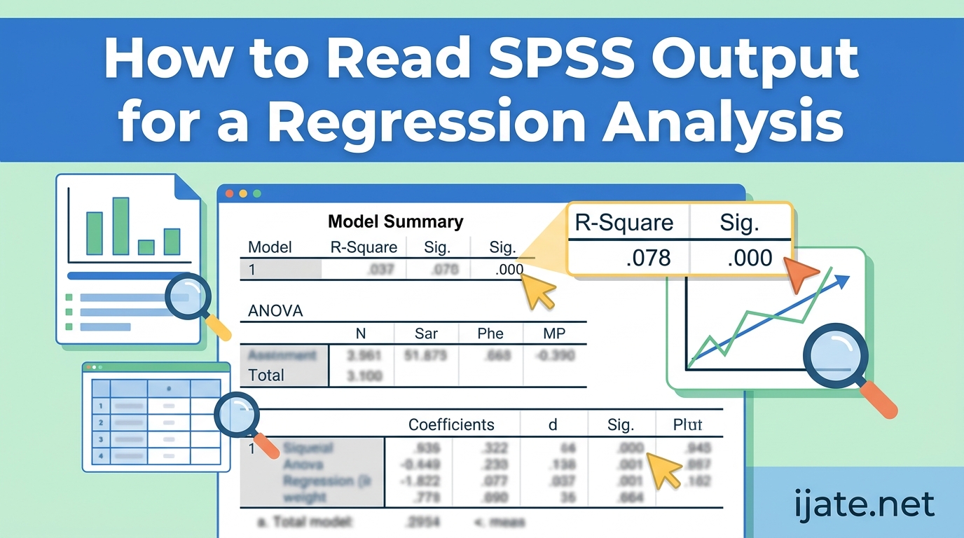
Learning how to read SPSS output for a regression analysis can feel overwhelming when you are staring at four tables filled with numbers, abbreviations, and statistical jargon. I remember running my first regression in SPSS and having no idea what R Square, Sig., or those B coefficients actually meant. If you are in that boat right now, you are in the right place.
This guide walks you through every table and every column in plain English. By the end, you will know how to determine whether your regression model is statistically significant, how much variance your predictors explain, and how to build the actual prediction equation from your output. Whether you are writing a thesis, a research paper, or just trying to understand your stats homework, I will cover everything you need with real examples and zero unnecessary complexity.
Table of Contents
Quick Reference: The Four Main SPSS Regression Output Tables
SPSS produces four core tables when you run a linear regression. Here is a fast overview of each one and what it tells you:
- Variables Entered/Removed – Shows which independent variables were included in your model and the method used (e.g., Enter, Stepwise). Confirms SPSS used the correct predictors.
- Model Summary – Reports R, R Square, Adjusted R Square, and the Standard Error of the Estimate. This tells you how well your model fits the data overall.
- ANOVA – Tests whether your regression model is statistically significant as a whole. Look at the F-ratio and the Sig. value (p-value) here.
- Coefficients – The most important table. Shows the intercept, each predictor’s B coefficient, standard error, Beta, t-value, Sig. (p-value), and 95% confidence intervals. This is where you determine which individual predictors matter.
If you only have 30 seconds, the short version is this: check the ANOVA table for overall significance, look at R Square in the Model Summary for model fit, then read the Coefficients table to see which predictors are significant and what their effects are.
How to Read SPSS Output for a Regression Analysis: Table 1 – Variables Entered/Removed
The first table SPSS generates is the Variables Entered/Removed table. It looks simple, but it serves an important purpose: confirming that SPSS actually used the variables you intended.
The table has columns for Variables Entered, Variables Removed, and Method. Under Method, you will usually see “Enter,” which means all independent variables were added to the model simultaneously. If you used stepwise regression, this table would show variables being added or removed in each step.
Take a moment to verify that every independent variable you intended to include appears under Variables Entered and that the Variables Removed column is empty (for a standard Enter method). This quick check can save you from interpreting results based on the wrong set of predictors.
SPSS adds superscript letters (a, b, c) to cells in this table. These footnotes typically tell you what your dependent variable was and what method was used. For example, you might see “a. Dependent Variable: Income” and “b. All requested variables entered.” These footnotes are worth reading because they confirm your analysis setup.
Table 2: Model Summary (R, R-Squared, Adjusted R-Squared)
The Model Summary table tells you how well your regression model fits the observed data. This is where you find some of the most commonly reported statistics in all of regression analysis.
What is R (the Multiple R)?
The first column, labeled R, represents the multiple correlation coefficient. This is the correlation between your observed dependent variable values and the values predicted by your regression model. R ranges from 0 to 1, with higher values indicating a stronger linear relationship.
In simple linear regression with one predictor, R equals the absolute value of the Pearson correlation between your predictor and outcome variable. In multiple regression with several predictors, R represents the combined correlation of all predictors with the outcome.
Interpreting R-Squared and Adjusted R-Squared
R Square (also written as R-squared or R2) is the proportion of variance in your dependent variable that is explained by your independent variables. It is expressed as a value between 0 and 1, but researchers typically report it as a percentage.
For example, an R Square of 0.75 means that 75% of the variation in your dependent variable can be explained by the predictors in your model. The remaining 25% is due to factors outside your model or random error.
What does an R-squared value of 0.9 mean? It means your model explains 90% of the variance in the dependent variable. That is a very high value, suggesting an excellent fit. However, be cautious: values that high can sometimes indicate overfitting, especially with many predictors and a small sample.
Adjusted R Square modifies R Square to account for the number of predictors in your model. Every time you add a predictor, regular R Square goes up slightly even if that predictor is useless. Adjusted R Square penalizes you for adding predictors that do not contribute meaningfully.
In practice, Adjusted R Square is always equal to or lower than regular R Square. If you are comparing models with different numbers of predictors, always use Adjusted R Square rather than regular R Square. A large gap between R Square and Adjusted R Square suggests some of your predictors may not be pulling their weight.
Standard Error of the Estimate
The last column in the Model Summary table is the Standard Error of the Estimate. This tells you, on average, how far your predicted values fall from the actual observed values in your dataset.
Think of it as the average prediction error in the original units of your dependent variable. If your dependent variable is measured in dollars and the Standard Error of the Estimate is 5,000, your predictions are off by about $5,000 on average. Smaller values are better.
This statistic is especially useful when you want to compare the predictive accuracy of models with different dependent variables, since R Square is unitless but the Standard Error of the Estimate is in the same units as your outcome.
Table 3: ANOVA Table (F-Value, Significance, df)
The ANOVA table answers one critical question: is your regression model statistically significant as a whole? Before you look at individual predictors, you need to know whether the overall model does a better job of predicting the dependent variable than simply using the mean.
Sum of Squares Explained
The ANOVA table contains three rows: Regression, Residual, and Total. Each row has a Sum of Squares value.
The Regression Sum of Squares represents the variation in your dependent variable that is explained by your model. The Residual Sum of Squares (sometimes called Sum of Squares for Error) represents the unexplained variation. The Total Sum of Squares is the sum of both and represents all variation in the dependent variable.
If your Regression Sum of Squares is large relative to the Residual Sum of Squares, your model is explaining a meaningful portion of the variance. This ratio is what the F-test evaluates.
Degrees of Freedom (df)
The df column shows degrees of freedom for each source of variance. For the Regression row, df equals the number of predictors in your model. For the Residual row, df equals your sample size minus the number of predictors minus 1 (N minus k minus 1).
The Total df equals your sample size minus 1. These degrees of freedom are used to calculate the Mean Square values and the F-ratio.
Mean Square and the F-Ratio
The Mean Square column is calculated by dividing each Sum of Squares by its corresponding degrees of freedom. The F-ratio is then computed by dividing the Regression Mean Square by the Residual Mean Square.
A larger F-ratio indicates that the variation explained by your model is large relative to the unexplained variation. But the F-ratio alone does not tell you if the result is significant. For that, you need the Sig. column.
The Sig. Column: Is Your Model Significant?
The Sig. column in the ANOVA table is the p-value for the overall F-test. This is the number that determines whether your regression model is statistically significant.
If Sig. is less than 0.05, your model is statistically significant. This means at least one of your predictors has a statistically significant relationship with the dependent variable. If Sig. is greater than 0.05, your model as a whole does not explain a significant portion of the variance, and you should reconsider your choice of predictors or your research design.
For example, if your ANOVA table shows F(2, 197) = 45.67, p = .001, your model is highly significant. The notation F(2, 197) tells you that the regression df was 2 (two predictors) and the residual df was 197 (200 participants minus 2 predictors minus 1).
One important caveat: a significant overall F-test does not tell you which specific predictors are significant. It only tells you that at least one predictor is. To identify which ones, you need the Coefficients table.
Table 4: Coefficients Table (B, Std. Error, Beta, t, Sig., 95% CI)
The Coefficients table is the heart of your SPSS regression output. This is where you find the specific effect of each individual predictor on your dependent variable. I consider this the most important table to understand.
Unstandardized Coefficients (B)
The first column under Unstandardized Coefficients is labeled B. These are the raw regression coefficients that tell you how much your dependent variable changes for each one-unit increase in that predictor, holding all other predictors constant.
For example, if the B coefficient for a predictor called “Years of Education” is 2,500 and your dependent variable is annual income, that means each additional year of education is associated with a $2,500 increase in income, controlling for other variables in the model.
The first row in the Coefficients table is usually labeled (Constant). This is the Y-intercept of your regression equation. It represents the predicted value of your dependent variable when all predictors equal zero. While the constant is necessary for building your prediction equation, it often has no practical interpretation because a value of zero for all predictors may not be meaningful.
Standard Error
The Std. Error column shows the standard error of each B coefficient. The standard error measures how precisely your sample estimates the true population coefficient.
Smaller standard errors indicate more precise estimates. The standard error is also used to calculate confidence intervals and t-statistics for each coefficient.
If a coefficient has a very large standard error relative to the B value, the estimate is imprecise and the predictor may not be statistically significant.
Standardized Coefficients (Beta)
The Beta column shows standardized coefficients. These are the B coefficients converted to a common scale so you can compare the relative importance of predictors measured in different units.
Beta coefficients are expressed in standard deviation units. A Beta of 0.45 means that a one standard deviation increase in that predictor is associated with a 0.45 standard deviation increase in the dependent variable.
Use Beta to compare the strength of predictors within the same model. The predictor with the largest absolute Beta value has the strongest relative effect on the dependent variable. However, do not use Beta for building prediction equations; use B instead.
t-Statistic
The t column shows the t-statistic for each coefficient. This is calculated by dividing each B coefficient by its standard error. The t-statistic tests whether each individual predictor is significantly different from zero.
A larger absolute t-value means the coefficient is more likely to be statistically significant. As a rough guide, absolute t-values greater than 2 often indicate significance, but you should always confirm with the Sig. column.
Sig. (p-value) for Individual Predictors
The Sig. column in the Coefficients table is the p-value for each individual predictor’s t-test. This tells you whether that specific predictor has a statistically significant relationship with the dependent variable, after controlling for all other predictors.
If Sig. is less than 0.05, that predictor is statistically significant. If Sig. is greater than 0.05, the predictor does not have a statistically significant unique contribution to predicting the dependent variable in your model.
For instance, if the Sig. value for “Years of Education” is .003, that predictor is significant at the .05 level (and even at the .01 level). If the Sig. value for “Age” is .215, age is not a significant predictor in this model.
Pay attention to the sign of the B coefficient alongside the p-value. A significant positive B means the predictor is associated with an increase in the dependent variable. A significant negative B means the predictor is associated with a decrease.
95% Confidence Intervals
The last two columns in the Coefficients table show the lower and upper bounds of the 95% confidence interval for each B coefficient. This range tells you that, with 95% confidence, the true population value of the coefficient falls somewhere between the lower and upper bounds.
If the confidence interval does not include zero, the coefficient is statistically significant at the .05 level. If the interval spans zero (for example, lower bound is -1.2 and upper bound is 3.5), the predictor is not significant.
Confidence intervals are valuable because they give you a range of plausible values rather than just a single point estimate. A narrow confidence interval means your estimate is precise. A wide interval suggests more uncertainty, often due to a small sample size or high variability in the data.
How to Build the Regression Equation from SPSS Output
One of the most common questions students ask is how to construct the actual regression prediction equation from SPSS output. It is straightforward once you know where to look.
The general form of a multiple regression equation is: Y = a + b1X1 + b2X2 + … + bkXk, where Y is the predicted value of the dependent variable, a is the constant (intercept), and b1 through bk are the unstandardized B coefficients for each predictor.
Here are the steps to build it:
- Open the Coefficients table in your SPSS output.
- Find the (Constant) row and note the value under the B column. This is your intercept (a).
- For each predictor, note the B value from the Unstandardized Coefficients column.
- Write out the equation: Y = constant + (B1 x Predictor1) + (B2 x Predictor2) + …
- Use unstandardized B coefficients, never Beta, for this equation.
For example, suppose your Coefficients table shows a Constant of 12,000, a B of 2,500 for Years of Education, and a B of 1,200 for Years of Experience. Your regression equation would be: Predicted Income = 12,000 + (2,500 x Years of Education) + (1,200 x Years of Experience).
Now you can plug in any combination of predictor values to get a predicted value for the dependent variable. Keep in mind that predictions are most reliable when the predictor values fall within the range observed in your original dataset.
Standardized vs Unstandardized Coefficients: What is the Difference?
The difference between standardized (Beta) and unstandardized (B) coefficients confuses many students. Here is a clear breakdown.
Unstandardized coefficients (B) describe the effect of each predictor in its original measurement units. Use B when you want to build a prediction equation, report practical effect sizes, or apply the model to real-world predictions. B coefficients change if you rescale a predictor (for example, switching from centimeters to meters).
Standardized coefficients (Beta) describe the effect of each predictor in standard deviation units. Because all predictors are on the same scale, you can compare Beta values directly to determine which predictor has the strongest relative effect. Beta does not change if you rescale a predictor.
Use Beta when you want to compare the importance of predictors within the same model. Use B when you want to make actual predictions or report effects in meaningful units. Never use Beta in the regression prediction equation.
One more consideration: Beta coefficients are affected by the variability of each predictor in your specific sample. A predictor with low variability may have a small Beta even if its B coefficient is substantial. Always interpret both in context.
Common Mistakes When Interpreting SPSS Regression Output
After working with students and reviewing dozens of regression analyses, I see the same interpretation mistakes repeatedly. Avoiding these will put you ahead of most people running SPSS regression for the first time.
Mistake 1: Confusing Overall Significance with Individual Significance
A significant F-test in the ANOVA table does not mean every predictor is significant. It means at least one predictor is significant. Always check the Sig. column in the Coefficients table for each individual predictor before drawing conclusions.
Mistake 2: Using Beta Instead of B in the Prediction Equation
The regression prediction equation requires unstandardized B coefficients. Using Beta produces incorrect predictions because Beta is on a standardized scale that does not correspond to the original units of your variables.
Mistake 3: Ignoring the Sign of the Coefficient
A statistically significant predictor with a negative B coefficient indicates an inverse relationship. As that predictor increases, the dependent variable decreases. Do not assume all significant predictors are positive relationships.
Mistake 4: Equating a Large R-Squared with a Good Model
A high R Square does not automatically mean your model is good or that your predictors are meaningful. It could reflect overfitting, especially with many predictors and a small sample. Always consider Adjusted R Square, sample size, and whether the predictors make theoretical sense.
Mistake 5: Interpreting Non-Significant Predictors
If a predictor’s Sig. value is above 0.05, you should not interpret its B coefficient as meaningful. The coefficient could be positive or negative purely due to random sampling variation. Report it as non-significant and move on.
Mistake 6: Assuming Causation
Regression analysis identifies associations, not causal relationships. Even if a predictor is highly significant, you cannot conclude it causes changes in the dependent variable without additional evidence from your research design.
How to Report SPSS Regression Results in APA Format
Reporting regression results in APA format requires specific information presented in a standard structure. Here is what you need and how to format it.
At minimum, your writeup should include: whether the overall model was significant (with F-statistic, degrees of freedom, and p-value), the R Square value, and the significant individual predictors (with B coefficients, t-values, p-values, and optionally confidence intervals).
Here is a template you can adapt: “A multiple linear regression was calculated to predict [dependent variable] based on [predictor 1] and [predictor 2]. A significant regression equation was found (F(df1, df2) = F-value, p = .xxx), with an R Square of .xxx. The predicted [dependent variable] is equal to [constant] + [B1] x [predictor 1] + [B2] x [predictor 2], where [predictor 1] is measured in [units]. [Predictor 1] was a significant predictor (B = xxx, t(df) = xxx, p = .xxx). [Predictor 2] was not a significant predictor (B = xxx, t(df) = xxx, p = .xxx).”
Here is a concrete example: “A multiple linear regression was calculated to predict income based on years of education and years of experience. A significant regression equation was found (F(2, 197) = 45.67, p < .001), with an R Square of .317. Participants’ predicted income is equal to 12,000 + 2,500 x years of education + 1,200 x years of experience. Years of education was a significant predictor (B = 2,500, t(197) = 8.32, p < .001). Years of experience was not a significant predictor (B = 1,200, t(197) = 1.45, p = .148).”
When reporting p-values, APA style uses three decimal places. Report exact p-values when possible, except when p is less than .001, in which case write p < .001. Report R Square and B coefficients to three decimal places as well.
Quick Interpretation Checklist
Use this checklist every time you need to interpret SPSS regression output. It covers the essential steps from top to bottom.
- Check the Variables Entered/Removed table to confirm your predictors were included correctly.
- Note the R Square value in the Model Summary to see what percentage of variance your model explains.
- Compare R Square and Adjusted R Square to check for overfitting or unnecessary predictors.
- Check the ANOVA table Sig. value to determine if the overall model is statistically significant (p < .05).
- In the Coefficients table, identify which predictors have Sig. values below .05 (those are significant).
- Note the direction (positive or negative) of each significant B coefficient.
- Use B coefficients and the Constant to build your regression prediction equation.
- Check the 95% confidence intervals to assess precision of your estimates.
- Report results in APA format using the template above.
FAQ’s
How to interpret regression results from SPSS?
How to read a regression analysis output?
How to interpret output in SPSS?
What does a R2 value of 0.9 mean?
Conclusion
Knowing how to read SPSS output for a regression analysis comes down to understanding four tables and a handful of key statistics. The Model Summary tells you how well your model fits the data through R Square and Adjusted R Square. The ANOVA table tells you whether the model as a whole is statistically significant. The Coefficients table tells you which specific predictors matter and how large their effects are.
The next time you run a regression in SPSS, work through the quick interpretation checklist above. Start with overall significance, then move to model fit, then examine individual predictors. With practice, reading these tables becomes second nature. If you are writing up your results for a thesis or paper, use the APA format template provided to structure your findings clearly and professionally.