
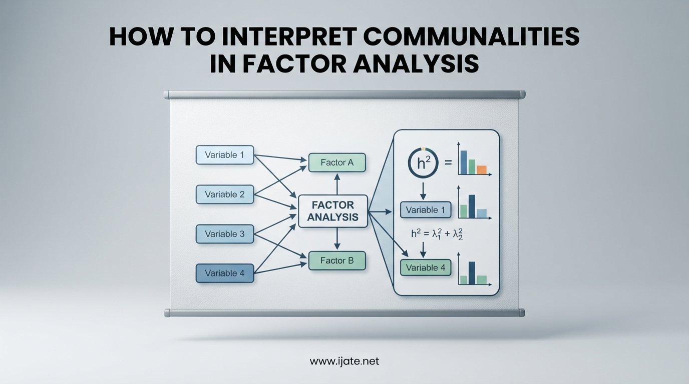
If you have ever stared at an SPSS communalities table and wondered whether your factor analysis actually worked, you are in the right place. Learning how to interpret communalities in factor analysis is one of the most common stumbling blocks for researchers running exploratory factor analysis for the first time. I have spent years working through factor solutions across psychometric scale development, survey validation, and social science research, and the communality column is always where the real story begins.
Communalities tell you how much of each variable’s variance your factors actually capture. They are the diagnostic check that tells you whether your factor solution is solid or whether you need to drop items, add factors, or rethink your extraction method. Yet most tutorials gloss over the practical interpretation and jump straight to rotation and factor loadings.
In this guide, I walk you through what communality means, how it is calculated, what counts as a good value, and how to read the SPSS communalities table step by step. I also cover R code, common mistakes, and the difference between initial and extraction communalities so you can confidently report your results.
Table of Contents
Quick Answer: What Is Communality in Factor Analysis?
Communality (denoted h-squared or h2) is the proportion of an observed variable’s variance that the extracted factors explain together. It ranges from 0 to 1, and it is calculated by summing the squared factor loadings for that variable across all retained factors. A value closer to 1 means the variable is well represented by the factor solution, while a value near 0 means the factors barely capture that variable.
In SPSS output, you will see two columns: Initial communality and Extraction communality. The initial value is the starting estimate placed on the diagonal of the correlation matrix before extraction, while the extraction value is the final communality after the factor solution has been computed. Comparing these two numbers tells you how much the estimation process shifted your variance explanation.
What Is Communality in Factor Analysis?
Communality represents the common variance a variable shares with all other variables through the underlying latent factors. Think of every observed variable in your dataset as having a total variance of 1 (when standardized). That total variance gets partitioned into two broad pieces: common variance and unique variance. Communality is the common variance piece.
Unique variance further splits into specific variance and error variance. Specific variance is variance that is reliable but unique to that single variable. Error variance is random measurement noise. So the full partitioning model is: total variance equals common variance plus specific variance plus error variance. Communality isolates only the common piece.
Mathematically, communality is the squared correlation between an observed variable and the linear combination of factors that predict it. If a variable loads strongly on one or more factors, those factors reproduce most of the variable’s behavior, and communality climbs toward 1. If the variable has weak or scattered loadings, communality drops.
This is why researchers care so much about communality. It tells you, variable by variable, whether your factor model is doing its job. A factor solution with uniformly high communalities means your factors capture the dataset well. A solution peppered with low communalities means some variables are not pulling their weight in the common factor structure.
One important nuance: communality is relational. A variable’s communality depends on the other variables in the analysis and the number of factors retained. Add or remove variables, and communalities shift. Change the number of factors, and communalities change again. This is why communality should always be interpreted in the context of a specific factor solution, not as an absolute property of the variable itself.
Communality vs Uniqueness
Uniqueness is the complement of communality. If communality is the proportion of variance explained by the factors, uniqueness is the proportion left unexplained. The formula is simple: uniqueness equals 1 minus communality.
So if a variable has a communality of 0.73, its uniqueness is 0.27. That 27 percent is the combination of specific variance and error variance that the factors do not capture. Researchers often report uniqueness alongside communality because the two numbers frame the same idea from opposite directions.
High uniqueness with low communality is a warning sign. It means the variable operates largely independently of the common factor structure, which may indicate poor measurement, a genuinely distinct construct, or a problematic item that should be removed.
Communality vs Eigenvalue
People often confuse communality with eigenvalue because both describe variance in factor analysis. The key difference is direction: communality is variance explained per variable, while eigenvalue is variance explained per factor.
Communality sums across factors for a single variable. Eigenvalue sums across variables for a single factor. If you add up all the communalities, you get the total variance explained by the entire factor solution. If you add up all the eigenvalues for retained factors, you get the same number. They are two perspectives on the same underlying variance accounting.
The Communality Formula and How It Is Calculated
The communality formula for variable j across k retained factors is: h-squared-j equals the sum of lambda-j-k squared, where lambda is the factor loading. In plain terms, you take every factor loading for that variable, square each one, and add them up.
Here is a manual calculation. Suppose variable X loads 0.80 on Factor 1, 0.30 on Factor 2, and 0.10 on Factor 3. Square each loading: 0.64, 0.09, and 0.01. Sum them: 0.74. The communality of variable X is 0.74, meaning the three factors together explain 74 percent of this variable’s variance.
Notice that the largest loading dominates the communality. A single strong loading of 0.80 already contributes 0.64 to the communality before any other factor is considered. This is why cross-loadings, even moderate ones, add only marginally to communality compared with a clean primary loading.
Negative loadings work the same way. Squaring a negative loading produces the same value as squaring its positive counterpart. A loading of minus 0.70 contributes 0.49 to communality, identical to a loading of positive 0.70. The sign tells you direction of relationship, but communality only cares about magnitude.
How Extraction Methods Affect Communality
The extraction method you choose changes how communalities are estimated, and this is a frequent source of confusion. Here is a comparison of the three most common methods.
Principal Components Analysis (PCA) starts every variable with an initial communality of 1.0 because PCA treats all variance as fair game. There is no distinction between common and unique variance in PCA. The diagonal of the correlation matrix is filled with 1s, meaning total variance is being decomposed, not just shared variance.
Principal Axis Factoring (PAF) starts with squared multiple correlations (SMC) as initial communalities on the diagonal. SMC values are typically well below 1.0, often in the 0.3 to 0.7 range depending on how intercorrelated your variables are. PAF then iteratively re-estimates communalities until they stabilize, producing final extraction communalities that reflect only common variance.
Maximum Likelihood (ML) extraction also estimates communalities but uses a different statistical criterion based on fitting the observed correlation matrix to a model-implied matrix. ML communalities can differ from PAF values, sometimes noticeably, especially with smaller samples.
The practical takeaway: PCA will almost always show higher communalities than PAF or ML for the same data, because PCA is partitioning total variance rather than just common variance. This is not a flaw in PCA. It is a definitional difference. If you are doing true common factor analysis for latent construct measurement, PAF or ML is the appropriate choice, and you should expect lower communalities as a natural consequence.
How to Interpret Communality Values
Interpreting communality values requires judgment, not just a rigid cutoff. However, there are widely used guidelines that give you a starting framework. I rely on the thresholds below, which draw on recommendations from Costello and Osborne (2005), Fabrigar and Wegener (2012), and common practice in psychometric scale construction.
Below 0.40 is considered low and potentially problematic. A variable with a communality under 0.40 shares less than 40 percent of its variance with the common factors. This variable is contributing more noise than signal to the factor solution and is a candidate for removal.
Between 0.40 and 0.50 is marginal. The variable is adequately represented but not strongly. If most of your variables sit in this range and the factor structure is otherwise clean, you can proceed, but keep an eye on these items during replication.
Between 0.50 and 0.70 is good. The factors explain half to three-quarters of the variable’s variance, which is solid for most social science applications. Variables in this range are pulling their weight.
Above 0.70 is excellent. The variable is strongly represented by the factor solution. When all or most variables reach this level, you likely have a clean, well-defined factor structure.
These thresholds are guidelines, not laws. In psychometric test construction, researchers sometimes accept communalities as low as 0.30 for items that load cleanly on a single factor and have strong theoretical justification. In other contexts, such as scale validation for high-stakes assessment, you might want every communality above 0.60.
Initial vs Extraction Communalities
The SPSS communalities table always shows two columns: Initial and Extraction. Understanding the difference is essential.
Initial communalities are the values placed on the diagonal of the correlation matrix before factor extraction begins. In PCA, these are always 1.0 because PCA analyzes total variance. In PAF, these are squared multiple correlations, which estimate how much each variable is predicted by all other variables combined.
Extraction communalities are the final values after the factor solution has been computed. In PCA, extraction communalities are the actual squared loading sums from the retained components. In PAF and ML, they reflect the iterative estimation process that refined the communalities during extraction.
The gap between initial and extraction communality tells a story. If initial SMC was 0.55 and extraction communality is 0.62, the factor solution improved the variance estimate for that variable. If extraction drops well below the initial SMC, the retained factors may be too few or the variable may not fit the common structure.
Forum users on r/statistics and r/spss frequently report confusion when they see initial communalities of 1.0 in PCA output. That 1.0 is not an estimate of common variance. It is a placeholder reflecting PCA’s treatment of all variance as analyzable. If you switch the same analysis to PAF, you will see initial communalities drop to SMC values, often between 0.3 and 0.7, which is the more honest starting estimate of shared variance.
Does Rotation Change Communalities?
No, rotation does not change communality values. This is one of the most common misunderstandings I see among students and early-career researchers.
Rotation redistributes the factor loadings across factors to achieve simpler, more interpretable structure. Varimax, oblimin, promax, and every other rotation method reassign how variance is allocated among factors. But the total squared loading sum for each variable, which is the communality, stays constant.
Think of it this way. Rotation rotates the factor axes but keeps the distance from each variable to the origin unchanged. That distance is the square root of communality. Whether you rotate orthogonally or obliquely, the communality for each variable remains identical before and after rotation.
This invariance is why you can interpret communalities confidently regardless of rotation choice. Your communality-based decisions about item quality hold whether you used varimax or oblimin.
Step-by-Step Worked Example: Interpreting Communalities in Practice
Let me walk you through a complete communality interpretation using a realistic scenario. Suppose you are validating a 10-item questionnaire measuring academic engagement. You collect responses from 300 participants and run exploratory factor analysis in SPSS using principal axis factoring with oblimin rotation.
After checking the correlation matrix and KMO measure (0.82, which is good), you retain three factors based on the scree plot and eigenvalues greater than 1. The communalities table appears in your SPSS output with Initial and Extraction columns for all 10 items.
Item 1 shows an initial SMC of 0.62 and an extraction communality of 0.71. This is excellent. The three factors explain 71 percent of this item’s variance, and the extraction improved on the initial estimate. Item 1 is strongly represented.
Item 2 shows an initial SMC of 0.48 and an extraction communality of 0.55. This is adequate. The item is reasonably well captured, though you would prefer to see it higher. No action needed.
Item 3 shows an initial SMC of 0.51 but an extraction communality of only 0.29. This is a red flag. The extraction dropped well below the initial estimate, meaning the three retained factors cannot adequately reproduce this variable’s shared variance. This item is a candidate for removal.
Item 4 shows an initial SMC of 0.36 and an extraction communality of 0.33. Both are low. This item barely shares variance with the other variables to begin with, and the factor solution confirms that weakness. Remove it.
After removing Items 3 and 4 and re-running the analysis, the remaining items show communalities between 0.52 and 0.79. The factor structure is now cleaner, with clear simple structure on the pattern matrix. This is the iterative process of using communalities to refine your factor solution.
The lesson: never accept your first factor solution blindly. Read the communalities table, identify weak items, remove them, and re-run. Each iteration should improve overall communality levels and clarify the factor structure.
Reading the SPSS Communalities Table Step by Step
Step 1: Locate the Communalities table in your SPSS output. It typically appears after the KMO and Bartlett’s test and before the Total Variance Explained table.
Step 2: Check the Initial column first. If you used PCA, every value will be 1.0. If you used PAF or ML, these are SMC values. Low initial communalities (below 0.40) signal weak inter-item correlations from the start.
Step 3: Move to the Extraction column. These are your final communality values. Compare each to the thresholds discussed earlier.
Step 4: Flag any variable with extraction communality below 0.40. Consider whether it loads cleanly on any factor in the pattern matrix. If it has a weak primary loading and low communality, remove it.
Step 5: Look at the overall pattern. If most variables have communalities above 0.60, your solution is strong. If many cluster between 0.40 and 0.50, consider whether you need more factors or a different extraction method.
Calculating and Inspecting Communalities in R
If you work in R, the psych package makes communality inspection straightforward. After running your factor analysis, the loadings object contains everything you need.
Use the fa function from the psych package: fa_result <- fa(mydata, nfactors = 3, rotate = "oblimin", fm = "pa"). This runs principal axis factoring with three factors and oblimin rotation.
To see communalities directly, access fa_result$communality. This returns a named vector of communality values for each variable. Sort them with sort(fa_result$communality) to quickly spot the lowest values.
To verify manually, square the loadings and sum across factors: rowSums(fa_result$loadings^2). This should match the communality vector exactly, confirming your understanding of the calculation.
Uniqueness is available via fa_result$uniquenesses, which equals 1 minus communality for each variable. Print both side by side for a complete variance accounting.
Common Mistakes When Interpreting Communalities
The most common mistake is treating initial communalities of 1.0 in PCA as meaningful estimates. They are not. PCA places 1.0 on the diagonal because it analyzes total variance, not common variance. If you want estimated communalities, use PAF or ML extraction.
Another frequent error is assuming that negative factor loadings reduce communality. They do not. Communality uses squared loadings, so a loading of minus 0.70 contributes exactly as much as positive 0.70. The sign indicates direction, not magnitude.
Researchers sometimes panic when extraction communalities are lower than initial communalities in PAF. A modest drop is normal and expected. The iterative estimation process refines the diagonal estimates, and the extraction values are the more accurate representation of common variance.
A subtle but important mistake is comparing communalities across different factor solutions without controlling for the number of factors. Adding factors almost always inflates communality because you are summing across more squared loadings. A four-factor solution will show higher communalities than a two-factor solution for the same data, even if the extra factors are not meaningful. Always interpret communality within a specific factor solution.
Finally, do not use communality as the sole criterion for item retention. A variable with marginal communality (say, 0.45) that loads cleanly and exclusively on one theoretically meaningful factor may be worth keeping. Conversely, a variable with high communality that cross-loads across three factors adds confusion. Pair communality interpretation with factor loading patterns, theoretical alignment, and reliability analysis.
FAQs
How do you interpret communality?
Communality ranges from 0 to 1 and represents the proportion of a variable’s variance explained by the extracted factors. Values above 0.70 are excellent, 0.50 to 0.70 are good, 0.40 to 0.50 are marginal, and below 0.40 suggests the variable is poorly represented and may need removal.
What do communalities mean in factor analysis?
Communalities indicate how much of each observed variable’s variance the common factors account for. A high communality means the variable shares substantial variance with other variables through the latent factors, while a low communality signals weak representation in the factor structure.
What is the difference between initial and extraction communalities?
Initial communalities are the starting values placed on the correlation matrix diagonal before extraction. In PCA these are always 1.0, while in PAF they are squared multiple correlations. Extraction communalities are the final values after the factor solution is computed and represent the actual variance each variable shares with the retained factors.
What do the extracted communalities in factor analysis represent?
Extracted communalities represent the proportion of each variable’s variance that the retained factors explain after the extraction process is complete. They are calculated as the sum of squared factor loadings for each variable across all retained factors.
Does rotation change communality values?
No. Rotation redistributes factor loadings among factors but does not change the total communality for any variable. The sum of squared loadings remains identical before and after rotation, whether you use an orthogonal method like varimax or an oblique method like oblimin.
Why are my communalities low in principal axis factoring?
PAF estimates only common variance, not total variance, so communalities are naturally lower than in PCA. Low communalities in PAF may indicate weak inter-item correlations, too few retained factors, or items that do not belong in the common factor structure.
Conclusion
Knowing how to interpret communalities in factor analysis gives you a diagnostic tool that goes far beyond simply reading factor loadings. Communality tells you, for every variable, whether your factor solution is capturing meaningful shared variance or leaving signal on the table.
Start with the extraction communalities. Flag anything below 0.40. Compare initial to extraction values to understand how your estimation method shaped the solution. Remember that rotation does not change communalities, that PCA inflates them relative to PAF and ML, and that negative loadings contribute just like positive ones when squared.
Pair your communality reading with factor loadings, theoretical judgment, and reliability checks. When you remove weak items and re-run the analysis, your communalities should rise and your factor structure should clarify. That iterative refinement is the heart of good exploratory factor analysis practice.