
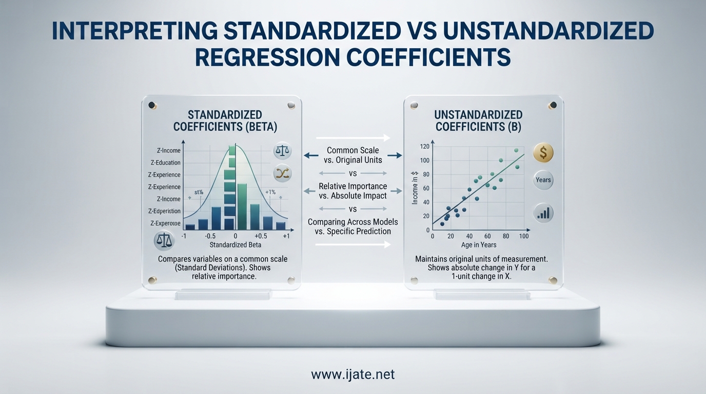
When you run a regression model in R, SPSS, or Python, the output returns two sets of coefficients for each predictor variable. An unstandardized regression coefficient, labeled as B, tells you how the outcome variable changes for each raw unit change in the predictor. A standardized regression coefficient, labeled as beta or Beta, tells you the same relationship but in units of standard deviations. Most researchers I speak with know both types exist but are unsure which one to report in their papers or which one to trust when making decisions.
This confusion matters because choosing the wrong coefficient type can lead to misleading conclusions in research publications, policy briefs, or business dashboards. In this guide, I will walk you through exactly what each coefficient represents. You will learn how to interpret each type in practice and how to decide which one to use for your specific situation.
The fundamental difference comes down to scale and units. Unstandardized coefficients work in the original measurement scale of your data. Standardized coefficients strip away the original units entirely by converting all variables to z-scores before running the regression. Neither coefficient type is universally better. They serve different analytical purposes, and understanding how to use both is essential for rigorous statistical work.
Table of Contents
How to Interpret Standardized Versus Unstandardized Regression Coefficients: Quick Comparison
The table below gives you a side-by-side view of the two coefficient types at a glance.
| Feature | Unstandardized Coefficient (B) | Standardized Coefficient (Beta) |
|---|---|---|
| Symbol in output | B | Beta or stdb |
| Units | Original scale (dollars, years, kg, etc.) | Standard deviations (unitless) |
| Core interpretation | Change in outcome per 1-unit change in predictor | Change in outcome per 1-SD change in predictor |
| Scale dependent? | Yes – changing units changes the coefficient | No – stays fixed regardless of unit changes |
| Best application | Real-world prediction, policy analysis, clinical interpretation | Comparing predictor importance, cross-study effect comparison |
| Intercept preserved? | Yes – meaningful on original scale | No – intercept is typically not reported |
| Can exceed 1.0? | Yes (rare in practice) | Yes (common with multicollinearity) |
| Binary predictors | Interpretable as group mean difference | Problematic – depends on class distribution |
Use this table as a quick reference as you read through the detailed sections that follow. Each row highlights a key distinction that affects how you should interpret and report your results.
What Are Unstandardized Regression Coefficients?
An unstandardized regression coefficient is the raw estimate produced directly by an ordinary least squares regression model. It appears in your software output as the column labeled B in SPSS, the coefficients section in R’s lm() output, or the coef() table in Python’s statsmodels library. The coefficient represents the average change in the dependent variable for a one-unit increase in the independent variable, holding all other predictors in the model constant.
Because the coefficient uses the original measurement units, a B of 2.5 carries direct real-world meaning. If your outcome is blood pressure measured in mmHg and your predictor is daily sodium intake in grams, then B = 2.5 means each additional gram of sodium is associated with a 2.5 mmHg higher blood pressure on average. This concrete interpretability makes unstandardized coefficients the natural choice when you need to explain results to non-technical audiences.
Hospital administrators, policy makers, and business leaders think in patient counts, dollars, and days rather than standard deviations. Unstandardized coefficients bridge that communication gap by keeping the results anchored in the language of the original measurement. The coefficient also directly answers causal or policy questions. If you are modeling how a $1,000 increase in per-pupil spending affects graduation rates, the unstandardized coefficient tells you the exact change in graduation percentage points per dollar. That is the kind of number a school board can act on immediately.
How to Interpret Unstandardized Coefficients in Practice
Reading an unstandardized coefficient follows a clear four-step process. First, identify the unit of measurement for the predictor variable. Second, read the B value as the expected change in the outcome for a one-unit shift in that predictor while holding all other variables constant. Third, check the sign: a positive B means the outcome rises as the predictor increases, while a negative B means it falls. Fourth, confirm the finding is statistically significant by examining the p-value, standard error, or confidence interval.
A coefficient can be small in raw magnitude but still highly significant if the standard error is proportionally small and your sample size is large. One situation that trips up many researchers is when the unstandardized coefficient appears near zero, such as 0.0003 or 0.02, and the researcher assumes the effect is trivial. In reality, the small B value simply reflects the scale of the predictor. When a variable is measured in very large units like dollars, population counts, or seconds, the raw coefficient will be tiny even when the relationship is strong.
I once reviewed a dataset where household income was recorded in exact dollar amounts. The regression returned B = 0.0003 for income predicting savings. The analyst initially concluded income had no effect. The truth was that each additional dollar of income was associated with a $0.0003 increase in savings. A $10,000 income increase corresponded to a $3 increase in savings, which was both economically meaningful and statistically significant. The near-zero B was purely an artifact of using dollar-level units rather than thousands of dollars. Rescaling income to thousands would have produced B = 3.0, which reads much more naturally without altering the underlying relationship at all.
What Are Standardized Regression Coefficients?
A standardized regression coefficient, often called a beta weight, is what you get when you convert every variable in the model to a z-score before running the regression. The z-score transformation subtracts the variable’s mean and divides by its standard deviation. After this conversion, each variable has a mean of exactly 0 and a standard deviation of exactly 1. When you run the regression on these standardized values, the resulting coefficients reflect how many standard deviations the outcome variable changes for a one-standard-deviation increase in the predictor.
The symbol for this coefficient is typically the Greek letter beta, though some software packages label it as Beta or stdb to distinguish it from the unstandardized B. The standardization process removes the original measurement units entirely, which makes standardized coefficients especially useful for comparing the relative strength of predictors that are measured on vastly different scales. If you want to know whether age in years or income in dollars has a stronger relationship with your outcome variable, you cannot compare their raw B values directly. Age might range from 18 to 80 while income ranges from $20,000 to $200,000. The different scales artificially distort the magnitude of the unstandardized coefficients.
Standardized coefficients put all predictors on the same footing by expressing everything in standard deviation units. This allows you to see which predictor moves the outcome more relative to its own variability in the sample. The key advantage is comparability across variables that would otherwise be incommensurable due to their different measurement scales.
How to Interpret Standardized Coefficients Correctly
Reading a standardized coefficient requires thinking in terms of standard deviation shifts rather than raw unit changes. A standardized beta of 0.45 means that a one-standard-deviation increase in the predictor is associated with a 0.45 standard-deviation increase in the outcome. Because all variables are on the same z-score scale, a larger absolute beta suggests that the predictor has a stronger relative effect compared to other predictors in the model. This makes standardized coefficients popular for ranking predictors by importance or for comparing effect sizes across studies that used different measurement instruments.
However, there is an important limitation that many researchers miss. Standardized coefficients are only fully comparable across predictors within the same model when those predictors have roughly similar distributions and variability. If one predictor is highly skewed and another is approximately normal, the standardization process does not completely eliminate the scale distortion. A standardized coefficient of 0.50 for a log-transformed predictor does not necessarily represent twice the effect of a standardized coefficient of 0.25 for a normally distributed predictor.
The absolute magnitude of a standardized beta is sensitive to the distribution shape and variability of the underlying variable. Treating standardized coefficients as universally comparable across different types of predictors is one of the most common errors I see in applied research. Always check the distribution and variability of your predictors before using standardized betas to rank their relative importance.
The Mathematical Relationship Between Standardized and Unstandardized Coefficients
The connection between the two coefficient types follows a precise mathematical rule. For a simple linear regression with a single predictor, the standardized coefficient equals the Pearson correlation coefficient between the predictor and the outcome. In multiple regression with several predictors, the relationship is more involved but still follows a clear formula. The standardized beta for any given predictor equals its unstandardized B multiplied by the ratio of the predictor’s standard deviation to the outcome variable’s standard deviation. In mathematical notation, beta_standardized equals B_unstandardized multiplied by sx divided by sy, where sx is the standard deviation of the predictor and sy is the standard deviation of the outcome variable.
This formula explains why changing the measurement scale of a variable changes its unstandardized coefficient but leaves the standardized coefficient unchanged. If you switch from measuring height in feet to measuring it in inches, the raw B value will shrink proportionally because each unit is smaller. But the ratio of sx to sy stays the same regardless of the unit choice, so the standardized beta remains fixed. This invariance to unit changes is one of the main reasons researchers prefer standardized coefficients for cross-study comparisons.
You can also reverse this conversion. If you have a standardized beta and need to reconstruct the unstandardized B, rearrange the formula: B equals beta times sy divided by sx. This reverse calculation is useful when you are reading a published paper that reports only standardized coefficients and you want to estimate the original effect size in real-world units. Knowing both the formula and the standard deviations of your variables lets you move freely between the two representations.
When to Use Unstandardized Coefficients
Unstandardized coefficients are the right choice whenever your goal involves prediction, communication, or decision-making in real-world units. If you are building a forecasting model for housing prices, you want the coefficients in dollars per square foot so that stakeholders can understand and act on the predictions. If you are evaluating a medical treatment, you want the effect size in mmHg, life-years, or percentage points so that clinicians can assess clinical significance.
Unstandardized coefficients also preserve the intercept term, which represents the expected value of the outcome when all predictors equal zero. That intercept is meaningful only when zero is a plausible value on the original measurement scale, something that standardization would destroy. Use unstandardized coefficients whenever you need to answer questions about actual changes in the world. A policy analyst modeling the effect of a minimum wage increase on employment needs the coefficient in jobs per dollar of wage change, not in standard deviations. A marketing team predicting sales from advertising spend needs the coefficient in dollars of revenue per dollar spent. In these applied contexts, the unstandardized coefficient is not just preferable. It is the only interpretation that makes sense to the people who will use your findings to make decisions.
When to Use Standardized Coefficients
Standardized coefficients shine when your analytical goal is to compare the relative importance of predictors that operate on very different scales. Suppose you are studying what drives employee productivity and your predictors include years of experience (ranging from 0 to 40), monthly training hours (ranging from 0 to 80), and a personality score on a 1-to-100 scale. The unstandardized B for years of experience might be 1.2, for training hours 0.8, and for personality 0.05. At first glance, experience appears to be the dominant factor. But those raw coefficients are misleading because the predictors have wildly different ranges and standard deviations. Standardizing them reveals the true relative contributions by putting all three predictors on the same z-score footing.
Standardized coefficients are also useful for comparing effect sizes across different studies or research groups. If two teams measure the same psychological construct using different instruments, their unstandardized coefficients will not be directly comparable. The standardized betas allow a rough comparison of effect magnitude across those studies. That said, I recommend caution here. Standardized coefficients are only comparable across models when the samples are drawn from similar populations and the variables have similar distributions. A standardized beta of 0.60 in a sample of college-educated professionals is not directly comparable to a standardized beta of 0.40 in a general population sample, because the restricted range in the college-educated group compresses variability and can inflate the apparent effect size.
Binary and Categorical Predictors: Special Considerations
Standardized coefficients become especially tricky when your model includes binary or categorical predictors. A binary variable coded as 0 and 1 has a standard deviation that depends entirely on how many observations fall into each category. If the split is perfectly balanced at 50-50, the standard deviation is exactly 0.5. If the split is 90-10, the standard deviation drops to approximately 0.3. The standardized coefficient for the same binary predictor will change depending on the class balance in your sample, even though the underlying relationship between the variable and the outcome has not changed at all.
This means the standardized beta for a binary predictor is not a pure measure of effect size. It is contaminated by the prevalence of the category in your particular sample. For this reason, many experienced statisticians recommend against using standardized coefficients for dummy variables or categorical predictors in most reporting situations. The unstandardized coefficient for a binary predictor has a clear and useful interpretation: it is the average difference in the outcome between the two groups. That interpretation is far more informative than a standardized beta that shifts whenever the sample composition changes.
If you do need to include a binary predictor alongside continuous predictors in a model where you also want standardized coefficients, the best approach is to report the unstandardized coefficient for the binary variable and the standardized coefficients for the continuous predictors. Add a clear footnote explaining why the two coefficient types are not on equal footing when binary variables are present. This transparency protects you from the criticism that you are comparing incomparable metrics.
Common Misconceptions and Pitfalls
Several misconceptions about regression coefficients circulate in online forums, statistics classrooms, and even published journal articles. Understanding these pitfalls will help you avoid common errors in your own analysis.
The Near-Zero Coefficient That Is Still Significant
One of the most frequent confusions I encounter is a researcher panicking because their unstandardized coefficient is 0.0003, 0.0005, or some similarly tiny number. The researcher concludes the effect is practically zero or meaningless. The coefficient is not meaningless. It simply reflects the measurement scale of the predictor. When a variable is recorded in very large units such as dollars, population counts, or seconds, the raw coefficient will be small in magnitude even when the relationship is strong and statistically significant.
Statistical significance depends on the ratio of the coefficient to its standard error, not on the raw magnitude of the coefficient itself. A B of 0.0003 with a tiny standard error and a large sample can be highly significant. A B of 5.0 with a large standard error and a small sample might fail to reach significance. Always examine the standard error, confidence interval, and p-value alongside the coefficient value before drawing conclusions about effect size.
Higher Standardized Beta Does Not Mean Higher Significance
Another common mistake is assuming that a predictor with a larger standardized beta must also have a smaller p-value or higher statistical significance. The magnitude of a coefficient and its statistical significance are fundamentally separate concepts. Statistical significance depends on the precision of the estimate, which is driven primarily by sample size and the residual variance in the data.
A standardized beta of 0.10 estimated from a sample of 50,000 observations can be extremely significant. A standardized beta of 0.60 estimated from a sample of 30 observations might not reach significance at all. Never judge the statistical importance of a predictor by the size of its coefficient alone. Always report and interpret the p-value or confidence interval alongside the standardized or unstandardized beta value.
Standardized Coefficients Can Exceed One
Some researchers operate under the mistaken belief that standardized coefficients must always fall between -1 and 1 because they resemble correlation coefficients. That constraint applies only to simple linear regression with a single predictor. In multiple regression with several predictors, standardized coefficients can exceed 1 in absolute value, especially when the predictors are highly correlated through multicollinearity.
A standardized beta of 1.3 or even 1.8 does not signal an error in your statistical software. It signals that the predictor has a strong association with the outcome after accounting for the other variables in the model, and the multicollinearity among predictors has amplified the coefficient. Treat values above 1 as valid outputs that require careful interpretation rather than as evidence that something went wrong in your analysis.
Reporting Guidelines for Research Papers
Academic journals have varying preferences about which coefficient type to include in regression tables. Many psychology, education, and social science journals using APA style express a preference for standardized betas because they allow readers to compare effect sizes across studies more easily. However, the current APA Publication Manual does not ban unstandardized coefficients. It recommends reporting unstandardized coefficients along with standard errors and confidence intervals as the primary results, and optionally including standardized coefficients as supplementary information.
If a journal editor specifically asks for standardized betas, you can comply while still providing the unstandardized B values in a footnote or appendix for full transparency. The safest and most defensible approach is to report both coefficient types whenever space allows. Present the unstandardized coefficients in your main regression table because they carry the original units and real-world meaning. Add a separate table with standardized coefficients for readers who want to compare your effect sizes to prior research.
If you are limited to a single table by journal word count constraints, report the unstandardized coefficients with their standard errors and confidence intervals, and include the standardized betas in parentheses next to each B value. This hybrid approach satisfies both the need for practical interpretation and the desire for cross-study comparability without sacrificing transparency.
Worked Example: Calculating Both Coefficient Types
Let me walk you through a complete worked example with real numbers. Imagine a simple linear regression where we predict university students’ final exam scores from the number of hours they studied per week. We have 50 students in our dataset. The mean study hours is 10 with a standard deviation of 4. The mean exam score is 75 with a standard deviation of 12. After running the regression, the unstandardized coefficient is B = 1.8.
Interpreting the unstandardized coefficient: each additional hour of study per week is associated with a 1.8-point increase in the final exam score. A student who studies 5 hours per week is predicted to score about 9 points lower than a student who studies 10 hours per week, assuming all other factors are equal. The unstandardized intercept would be around 57, meaning a student who does not study at all is predicted to score 57 points.
Now let us convert to the standardized coefficient using the formula. The standardized beta equals B_unstandardized multiplied by the ratio of the predictor standard deviation to the outcome standard deviation. That is 1.8 times (4 divided by 12). The ratio 4/12 equals 0.333. Multiplying 1.8 by 0.333 gives a standardized beta of approximately 0.60.
Interpreting the standardized coefficient: a one-standard-deviation increase in study hours is associated with a 0.60 standard-deviation increase in exam score. Since both variables are roughly normally distributed in this example, this tells us that study habits have a moderately strong relationship with exam performance. The standardized beta of 0.60 also makes it easy to compare this effect to other predictors if we expanded the model to include prior GPA, attendance rate, or socioeconomic status, because all coefficients would then be on the same standardized z-score scale.
To reverse the calculation, if you only had the standardized beta of 0.60 and wanted to reconstruct the unstandardized B, you would compute B equals beta times sy divided by sx. That is 0.60 times 12 divided by 4, which equals 1.8. The round-trip conversion confirms that both representations describe the same underlying relationship, just expressed in different units. The key insight is that the two numbers are mathematically linked. Knowing one and the standard deviations of both variables lets you compute the other exactly.
Computing Standardized Coefficients in R
If you use R for your analysis, computing standardized coefficients is straightforward with the scale() function. You create standardized versions of both variables by applying scale(), then run the regression on the standardized data. The resulting coefficient is the standardized beta. Alternatively, you can compute it directly from an unstandardized model using the formula beta equals B times the ratio of standard deviations.
Many R packages including lm.beta and QuantPsyc offer built-in functions to extract standardized coefficients directly from a standard lm() object without manually rescaling the data. In SPSS, standardized coefficients appear automatically in the output table labeled Beta alongside the unstandardized B coefficients. There is no need for extra syntax. In Python’s statsmodels library, you can standardize your variables using the StandardScaler from scikit-learn before fitting the model, or compute the standardized betas post-hoc using the formula approach. In all three platforms, the underlying mathematics is identical. The choice of software does not change the interpretation of the results.
Frequently Asked Questions
What is an unstandardized regression coefficient?
An unstandardized regression coefficient, labeled as B in regression output, represents the average change in the dependent variable for a one-unit increase in the independent variable while holding other predictors constant. It is expressed in the original measurement units of the variables.
Should I use standardized or unstandardized coefficients in regression?
Use unstandardized coefficients when you need real-world predictions, policy decisions, or communication in original units. Use standardized coefficients when comparing relative importance across predictors measured on different scales or when combining results across studies. In research reports, consider providing both for transparency.
How to calculate standardized regression coefficients from unstandardized?
Multiply the unstandardized coefficient B by the ratio of the predictor standard deviation to the outcome standard deviation. The formula is beta = B times (sx / sy), where sx is the standard deviation of the predictor and sy is the standard deviation of the dependent variable.
Do you report standardized or unstandardized betas APA?
APA style recommends reporting unstandardized coefficients with standard errors and confidence intervals as the primary results. Standardized betas can be included as supplementary information for cross-study comparison. Always check the specific guidelines of your target journal, as preferences vary by field.
The right choice between standardized and unstandardized regression coefficients depends entirely on your analytical goal. If you are predicting outcomes, explaining effects to stakeholders, or making policy decisions, stick with unstandardized coefficients. They keep the results in the original units where the meaning is clear and actionable. If you are comparing the relative importance of predictors on different scales, building a composite index, or combining results across studies, standardized coefficients are the better tool.
The best practice in academic research is to report both types whenever possible. Present the unstandardized coefficients as your primary results because they carry the original units and practical meaning. Add a supplementary table with standardized betas for readers who want to compare your effect sizes to prior work. This transparent approach lets your audience interpret the findings in whatever frame of reference suits their needs, and it protects you from the criticism that you cherry-picked the coefficient type that made your results look better.