
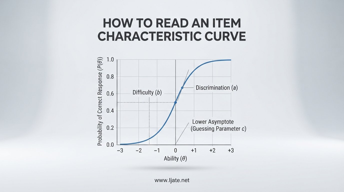
If you have ever stared at an S-shaped curve in a psychometrics textbook and wondered what it actually tells you, you are in the right place. Learning how to read an item characteristic curve is one of the most practical skills in item response theory (IRT), and it unlocks the ability to evaluate test items at a glance. Whether you are a graduate student working through a measurement course, a test developer reviewing item statistics, or a researcher running IRT models in R, the ICC is your primary diagnostic tool.
An item characteristic curve (ICC) plots the probability of a correct response against a test-taker’s underlying ability level, called theta. The curve rises from left to right because higher-ability test-takers are more likely to answer correctly. Once you understand the three parameters that shape the curve, you can read almost any ICC in seconds.
In this guide, I will walk you through every component of the ICC, from the axes and parameters to the differences between 1PL, 2PL, and 3PL models. I will also cover how to spot good, poor, and problematic items, why ICCs sometimes cross each other, and how to apply this knowledge in real test development work. By the end, you will have a clear, repeatable process for reading any item characteristic curve you encounter.
Table of Contents
Quick Overview: How to Read an ICC in 5 Steps
Here is the fastest way to read an item characteristic curve, broken into five steps you can apply every time.
Check the horizontal axis (theta). The X-axis represents ability, typically ranging from -3 to +3 logits. Values on the left indicate lower ability, and values on the right indicate higher ability.
Check the vertical axis (probability). The Y-axis shows the probability of a correct response, ranging from 0 to 1. The curve always rises from left to right in a monotonic S-shape.
Find the inflection point. The steepest part of the curve is where the item discriminates most effectively between ability levels. The horizontal position of this point tells you the item’s difficulty.
Check the lower asymptote. If the curve starts above zero on the left, that floor represents the guessing parameter. A curve starting near zero means low-ability test-takers have almost no chance of answering correctly by guessing.
Assess the slope. A steep slope means the item strongly differentiates between ability levels. A flat slope means the item discriminates poorly and may need revision.
These five steps form the foundation of ICC interpretation. The rest of this guide expands each step with the theory and parameters behind them.
What Is an Item Characteristic Curve?
An item characteristic curve is a graphical representation in item response theory that shows the relationship between a test-taker’s ability level and the probability that they will answer a specific item correctly. It is sometimes called an item response function or item response curve. The ICC is the visual output of a logistic model fitted to response data, and it gives you an immediate, intuitive picture of how an item behaves across the entire ability range.
The concept traces back to the foundational work of psychometricians like Frederic Lord and Allan Birnbaum in the mid-20th century, building on earlier work by Ledyard Tucker in 1946. The curve became central to IRT because it captures something classical test theory could not: how an item performs at every point along the ability continuum, not just on average.
ICCs are used extensively in educational testing, psychological assessment, health outcome measurement, and survey development. Any time a test or instrument needs to measure a latent trait, such as mathematical ability, depression severity, or patient-reported health status, ICCs help developers evaluate whether each item is doing its job.
Important disambiguation: The abbreviation ICC has two common meanings in statistics. In item response theory, it stands for item characteristic curve. In other contexts, particularly reliability analysis, ICC stands for intraclass correlation coefficient, which is a completely different concept measuring agreement between raters or measurements. This guide covers only the item characteristic curve.
Understanding the Axes of an ICC
Every ICC has two axes, and understanding them is the first step in reading the curve.
The Horizontal Axis: Ability (Theta)
The X-axis represents the latent trait or ability being measured, denoted by the Greek letter theta. Theta is typically scaled in logits (log-odds units) and centered at zero for the population mean. Most ICCs display a range from about -3 to +3, which covers roughly 99 percent of a normally distributed population.
Negative theta values represent below-average ability. Positive theta values represent above-average ability. A theta of zero represents the average test-taker. Because theta is a latent trait, it cannot be directly observed. It is estimated from response patterns using maximum likelihood or Bayesian estimation methods.
The Vertical Axis: Probability of Correct Response
The Y-axis represents the probability that a test-taker at a given ability level will answer the item correctly. This probability, written as P(theta), ranges from 0 to 1. The curve always increases from left to right, reflecting the assumption of monotonicity: higher ability should never decrease the probability of a correct response.
If you pick any theta value on the X-axis and trace vertically to the curve, then horizontally to the Y-axis, you get the exact probability of a correct response for someone at that ability level. This is the fundamental reading operation for any ICC.
The Three Parameters: a, b, and c
Every ICC is shaped by up to three parameters. Understanding these parameters is the heart of learning how to read an item characteristic curve.
The Discrimination Parameter (a)
The a parameter controls how steeply the curve rises at its inflection point. It measures how well the item differentiates between test-takers of different ability levels. A high a value produces a steep, sharp S-curve, meaning the item sharply separates those who know the content from those who do not. A low a value produces a gradual, flat curve, meaning the item discriminates poorly.
Typical a values range from about 0.5 to 2.0 in well-functioning tests. An item with a near zero or negative is seriously flawed and should be removed or rewritten. In the 1PL and Rasch models, the a parameter is fixed at 1.0 for all items, meaning every item is assumed to discriminate equally well.
The Difficulty Parameter (b)
The b parameter indicates where along the theta scale the curve is centered. It tells you how difficult the item is. A b value near zero means the item is targeted at average-ability test-takers. A positive b means the item is difficult, requiring above-average ability for a 50 percent chance of success. A negative b means the item is easy.
Here is a critical point that trips up many students. In the 1PL and 2PL models, the b parameter represents the theta value at which the probability of a correct response is exactly 0.50. But in the 3PL model, this is no longer true. Because the guessing parameter raises the lower asymptote, the 50 percent probability point shifts. In a 3PL model, the b parameter still indicates the location of the inflection point, but the probability at that point is (1 + c) divided by 2, not 0.50.
Common misconception callout: Many textbooks and online resources state that b is always the point where probability equals 50 percent. This is only correct for 1PL and 2PL models. If you are working with a 3PL model and the guessing parameter c is greater than zero, the b parameter does not correspond to the 50 percent probability point. Always account for the lower asymptote when interpreting difficulty in a 3PL framework.
The Guessing Parameter (c)
The c parameter represents the lower asymptote of the curve. It captures the probability that a very low-ability test-taker will answer correctly by guessing. On a multiple-choice item with four options, the theoretical minimum for c is 0.25, though empirically estimated c values often fall between 0.10 and 0.35.
When c is greater than zero, the curve does not start at the bottom of the Y-axis. Instead, it levels off at the c value on the far left. This creates a floor effect. In the 1PL and 2PL models, c is fixed at zero, meaning no guessing is assumed and the curve drops all the way to the bottom.
The IRT Models: 1PL, 2PL, and 3PL
The shape of an ICC depends on which IRT model you use. Three models dominate practice, and each adds one more parameter.
The 1PL Model (Rasch Model)
The one-parameter logistic model, also called the Rasch model, uses only the difficulty parameter b. The discrimination parameter is fixed at 1.0 for all items, and the guessing parameter is fixed at zero. This produces a family of parallel S-curves that differ only in their horizontal position. Easy items sit on the left, difficult items sit on the right, but every curve has the same shape.
The 1PL model is valued for its simplicity and its property of specific objectivity, which means item comparisons do not depend on which test-takers you use. The logistic equation for the 1PL is P(theta) equals 1 divided by (1 plus e raised to the power of negative (theta minus b)). The result is a clean sigmoid curve centered at theta equals b with probability 0.50 at that point.
A common distinction: the Rasch model and the 1PL model are nearly identical mathematically but differ philosophically. Rasch practitioners treat the model as a definitional standard that the data must fit, while 1PL practitioners treat it as a tool to fit to data.
The 2PL Model
The two-parameter logistic model adds the discrimination parameter a to the difficulty parameter b. Now each item can have both its own steepness and its own location. This produces curves that vary in both shape and position. Some items will be steep and discriminating, others will be flatter.
The 2PL equation is P(theta) equals 1 divided by (1 plus e raised to the power of negative a times (theta minus b)). The a parameter multiplies the entire exponent, scaling how quickly the curve transitions from low to high probability.
The 2PL model is the most commonly used model in practice for many testing programs. It captures real differences in item quality without the complexity and estimation difficulty of the guessing parameter.
The 3PL Model
The three-parameter logistic model adds the guessing parameter c on top of a and b. The full equation is P(theta) equals c plus (1 minus c) divided by (1 plus e raised to negative a times (theta minus b)). This means the curve starts at c on the left, rises through an S-shape, and approaches 1.0 on the right.
The 3PL model is most appropriate for multiple-choice items where guessing is plausible. However, it requires larger sample sizes to estimate reliably, and the c parameter can be unstable or fail to converge. Many practitioners prefer the 2PL unless there is strong evidence that guessing is a significant factor.
When you compare the three models, the progression is straightforward. The 1PL fixes a at 1 and c at 0. The 2PL frees a but keeps c at 0. The 3PL frees both a and c. More parameters mean more flexibility but also more data requirements and more potential for estimation problems.
Classical Test Theory vs Item Response Theory
To appreciate why ICCs matter, it helps to understand what they replace. Classical test theory (CTT) has been the dominant framework for test analysis for decades, and it still has its place. But IRT, powered by ICCs, offers advantages that CTT cannot match.
In CTT, item difficulty is the proportion of test-takers who answered correctly, often called the p-value. Item discrimination is a correlation between item score and total test score. Both statistics depend on the specific sample of test-takers you happen to have. A difficult item in a high-ability sample might look easy, and vice versa.
In IRT, item parameters are estimated independently of the sample, and ability is estimated independently of the specific items administered. This property, called parameter invariance, means the ICC describes the item’s behavior universally. The same ICC applies whether the item is given to low-ability or high-ability test-takers.
CTT provides single summary statistics for items. IRT provides a full curve showing performance at every ability level. That curve lets you see exactly where an item works well and where it breaks down, which is invaluable for test construction and adaptive testing.
How to Read an Item Characteristic Curve Step by Step
Now let me walk you through the complete process of reading an ICC. This is the practical method I use whenever I review item analysis output.
Step 1: Identify the Model Used
Before reading the curve, determine which IRT model generated it. A 1PL curve will always have the same shape, shifted left or right. A 2PL curve can vary in steepness. A 3PL curve may not start at zero on the Y-axis. Knowing the model tells you what to expect and which parameters to look for.
Step 2: Read the Difficulty
Find the inflection point, which is where the curve is steepest. Drop a vertical line from that point to the X-axis. The theta value at that location is the b parameter. If b is negative, the item is relatively easy. If b is positive, the item is relatively difficult. A b near zero targets average test-takers.
For 1PL and 2PL models, the probability at the inflection point is 0.50. For a 3PL model with guessing, look up the c value first, then calculate the probability at the inflection as (1 plus c) divided by 2.
Step 3: Read the Discrimination
Examine the steepness of the curve at the inflection point. A steep, sharp transition means high discrimination. The item cleanly separates those who can from those who cannot. A gradual, gentle slope means low discrimination. The item fails to distinguish between ability levels effectively.
Visually, compare the curve to a 45-degree reference line. If the curve is much steeper than 45 degrees at the inflection, discrimination is strong. If it is much flatter, discrimination is weak.
Step 4: Read the Guessing
Look at the far left of the curve. If the curve flattens out above the X-axis, that floor is the c parameter. The height of that floor tells you the guessing probability. If the curve drops all the way to near zero, there is no meaningful guessing parameter, and you are likely looking at a 1PL or 2PL model.
Step 5: Evaluate Overall Item Quality
Combine your readings into an overall judgment. A strong item has a steep slope, a difficulty matched to the target population, and minimal guessing influence. A weak item has a flat slope, a difficulty far from the population mean, or a high guessing floor. Flag weak items for revision or removal.
This five-step process works on every ICC you will encounter. With practice, you can complete all five steps in under a minute per item.
Visual Interpretation: Good, Poor, and Problematic ICCs
Once you can read individual parameters, the next skill is classifying items by their overall curve shape. Psychometricians commonly sort ICCs into four categories.
Good ICCs
A good ICC has a steep slope, indicating strong discrimination. The curve rises sharply from near zero to near one over a narrow theta range. The inflection point falls within the range of ability levels the test is designed to measure. There is little to no guessing floor, or if one exists, it is modest and accounted for by a 3PL model.
Good items efficiently separate test-takers across the relevant ability range. They contribute maximum information at the difficulty level where the test needs precision.
Limited Discrimination ICCs
A limited discrimination ICC has a noticeably flatter slope than a good ICC. The curve still rises monotonically from left to right, but the transition is gradual. These items discriminate in the right direction but do not separate ability levels sharply.
Limited discrimination items are not necessarily broken, but they contribute less information than steeper items. They may be retained if the test needs broad coverage, but they should not dominate the item pool.
Poor ICCs
A poor ICC is nearly flat across the entire theta range. The probability of a correct response barely changes from low to high ability. These items fail the fundamental purpose of measurement: they do not differentiate between test-takers who know the content and those who do not.
Poor items should be removed from the test. They add testing time without adding measurement value.
Problematic ICCs
A problematic ICC violates the assumption of monotonicity. Instead of rising steadily from left to right, the curve may dip, flatten and rise again, or even decrease at some points. This signals a serious issue, such as a miskeyed item, a confusing distractor that trips up high-ability test-takers, or a multidimensional item that is measuring something other than the intended trait.
Problematic items must be investigated and corrected or removed. They can distort ability estimates and undermine test validity.
Why ICCs Cross and What It Means
One of the most confusing phenomena for students is when two ICCs intersect. In a 1PL model, ICCs never cross because all items share the same discrimination parameter. The curves are parallel, differing only in horizontal position. But in 2PL and 3PL models, items can have different discrimination values, and their curves can cross.
When ICCs cross, the relative difficulty of the two items depends on the ability level. At one theta value, item A may be easier than item B. At a different theta value, the order reverses. A high-discrimination item that is difficult for average test-takers may actually be easier than a low-discrimination item for very high-ability test-takers.
This crossing matters because it means you cannot rank items by difficulty in a simple, universal order. The difficulty ordering changes across the ability spectrum. Test developers need to consider where their target population falls on the theta scale when selecting items.
Crossing ICCs are not necessarily a problem. They are a natural consequence of allowing items to have different discrimination parameters. But they do complicate interpretation, and they are a frequent source of confusion for students learning IRT for the first time.
The Item Information Function
Closely related to the ICC is the item information function. While the ICC tells you the probability of a correct response, the item information function tells you how much measurement precision the item provides at each ability level.
Information is highest where the ICC is steepest, near the inflection point. This makes sense: the item discriminates most effectively where the probability is changing most rapidly. Information drops to near zero at the extremes of the theta scale, where the curve is flat at the top or bottom.
The test information function is the sum of all item information functions. It shows the total precision of the test at every ability level. Test developers use this function to ensure the test provides adequate measurement precision across the range of abilities they care about.
If you are building a test for a specific purpose, such as a certification exam with a pass-fail cut score, you want maximum test information near that cut score. ICCs and information functions together guide the selection of items that deliver precision where it matters most.
Applications of ICCs in Test Development
ICCs are not just academic exercises. They drive real decisions in test construction and validation.
Item selection. Test developers use ICCs to choose items that target specific ability ranges. For a test measuring a broad population, you want items distributed across the theta scale. For a screening test with a specific cut point, you want items clustered around that difficulty level.
Item revision. When an ICC reveals poor discrimination or an unexpected guessing floor, developers can revise the item. A flat curve might prompt rewriting a confusing stem. A high guessing floor might mean the distractors are too obviously wrong.
Differential item functioning (DIF) analysis. By plotting separate ICCs for different demographic groups, developers can detect items that function differently for different populations. If the ICCs for men and women diverge significantly, the item may be biased and require review.
Computerized adaptive testing (CAT). CAT systems use ICCs and information functions in real time to select the next item that will provide the most information given the test-taker’s current ability estimate. This is what allows adaptive tests to achieve high precision with fewer items than fixed-form tests.
Test equating. When multiple forms of a test are administered, ICCs help place items on a common scale so scores can be compared fairly across forms. This is essential for high-stakes testing programs that release new forms regularly.
How to Interpret an Item Characteristic Curve: Quick Reference
Here is a concise summary you can return to whenever you need a refresher on ICC interpretation.
An item characteristic curve shows the probability of a correct response across the ability spectrum. Items that are difficult are shifted to the right of the ability scale, indicating the higher ability of the respondents who endorse them correctly. Items that are easier are shifted to the left of the ability scale. The steepness of the curve tells you how well the item discriminates, and the lower asymptote tells you how much guessing contributes to correct responses.
Read the curve left to right: locate the inflection point for difficulty, check the slope for discrimination, and check the floor for guessing. Compare multiple ICCs to see how items differ across the ability range. Flag flat curves for revision and non-monotonic curves for investigation.
FAQs
How to interpret an item characteristic curve?
To interpret an ICC, read the curve left to right. The horizontal position of the steepest point tells you the item difficulty (b parameter). The steepness at that point tells you the discrimination (a parameter). The height where the curve flattens on the far left tells you the guessing probability (c parameter). Items that are difficult to endorse are shifted to the right of the scale, while easier items are shifted to the left.
What is the difference between 1PL, 2PL, and 3PL models?
The 1PL (Rasch) model uses only the difficulty parameter, fixing discrimination at 1.0 and guessing at zero. The 2PL model adds a free discrimination parameter so each item can have its own slope. The 3PL model adds a guessing parameter so the curve can have a lower asymptote above zero. More parameters provide more flexibility but require larger sample sizes to estimate reliably.
What does the b parameter mean on an item characteristic curve?
The b parameter is the difficulty parameter. It indicates the theta value at which the curve is steepest. In 1PL and 2PL models, this is the point where the probability of a correct response is exactly 0.50. In the 3PL model with guessing, the probability at the inflection point is (1 plus c) divided by 2, not 0.50. A positive b means the item is difficult, and a negative b means the item is easy.
Why do item characteristic curves cross?
ICCs cross in 2PL and 3PL models because items have different discrimination parameters. When two curves have different slopes, they can intersect at some theta value. At that crossing point, the relative difficulty of the two items reverses. This means the difficulty ordering of items depends on the ability level of the test-takers. In the 1PL model, curves never cross because all items share the same discrimination.
What is a good fit in IRT?
A good fit in IRT means the chosen model (1PL, 2PL, or 3PL) accurately reproduces the observed response patterns. Researchers evaluate fit using statistics like the chi-square item fit index, the standardized residual, and information criteria such as AIC and BIC. A well-fitting model produces ICCs that closely match the empirical proportions of correct responses at each ability level, with no systematic deviations.
Is the item characteristic curve the same as the intraclass correlation coefficient?
No. Both are abbreviated ICC, but they are completely different concepts. The item characteristic curve is a graphical plot in item response theory showing the probability of a correct response against ability. The intraclass correlation coefficient is a reliability statistic measuring agreement between raters or repeated measurements. They share an abbreviation but have no mathematical or conceptual relationship.
Conclusion
Learning how to read an item characteristic curve gives you a powerful diagnostic tool for evaluating test items. The ICC tells you at a glance how difficult an item is, how well it discriminates between ability levels, and how much guessing contributes to correct responses. By reading the curve’s position, slope, and floor, you can make informed decisions about which items to keep, revise, or discard.
Start with the five-step process: check the axes, find the inflection point, read the difficulty, assess the slope, and check the guessing floor. Then classify each item as good, limited, poor, or problematic based on its overall curve shape. Apply this method consistently, and ICC interpretation will become second nature in your psychometric work.