How to Read Post-Hoc Test Results After an ANOVA? (2026 Guide)

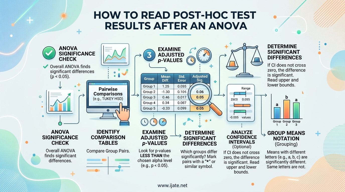
You ran an ANOVA, got a significant F-statistic, and now you are staring at a post hoc output table wondering what diff, lwr, upr, and p adj actually mean. Learning how to read post-hoc test results after ANOVA is the skill that separates someone who clicks through software menus from someone who can actually draw conclusions from their data. ANOVA tells you that at least one group mean differs from the others, but it does not tell you which ones. That is where post hoc tests come in.

In this guide, I will walk you through every column of a post hoc output table, break down what each number means, and show you how to decide whether a pairwise difference is significant. I will cover Tukey HSD, Bonferroni, Scheffe, Holm, and Dunnett, with worked examples from R, SPSS, and Python. By the end, you will be able to look at any post hoc output and translate it into a plain English conclusion.

Quick answer: A post hoc result is statistically significant when the adjusted p-value (p adj) is below 0.05 or when the confidence interval for the mean difference excludes zero. If either condition holds, the two groups being compared have significantly different means. If the confidence interval includes zero or p adj exceeds 0.05, you cannot conclude a significant difference exists between those specific groups.

What Is ANOVA and Why It Is Not Enough

ANOVA (Analysis of Variance) is an omnibus test that compares three or more group means simultaneously. It produces an F-statistic and a p-value that tell you whether at least one group mean differs from the rest. A significant ANOVA result (typically p less than 0.05) means you reject the null hypothesis that all group means are equal.

Here is the catch. The significant F-statistic does not identify which groups differ from which. If you have four treatment groups and your ANOVA is significant, you know that somewhere among those four groups, at least one pair has different means. But you do not know if Group A differs from Group B, or if Group C differs from Group D, or if only Group A stands apart from all others.

This is why ANOVA alone is insufficient for drawing specific conclusions about group differences. You need a follow-up procedure to pinpoint exactly which pairs of groups have significantly different means. That follow-up procedure is a post hoc test.

Think of ANOVA as a smoke detector. It tells you there is a fire somewhere in the building, but not which room. Post hoc tests are the investigation that follows, room by room, until you find the source.

What Are Post Hoc Tests and When to Use Them

Post hoc tests are pairwise comparison procedures performed after a significant ANOVA result. The phrase “post hoc” is Latin for “after this,” meaning these tests are conducted only after the omnibus ANOVA has detected a significant overall effect. Each post hoc test compares every possible pair of group means (or a specific subset) while adjusting for the increased risk of false positives that comes from running many comparisons.

You should run a post hoc test when your ANOVA produces a statistically significant F-statistic. At that point, you know that differences exist somewhere among your groups, and post hoc tests will identify the specific pairs that differ. This is the standard workflow for one-way ANOVA, two-way ANOVA (for significant main effects or interactions), and repeated measures ANOVA.

You should NOT run a post hoc test when your ANOVA is not significant. If the omnibus test fails to detect an overall effect, proceeding to pairwise comparisons is statistically inappropriate in most frameworks. A non-significant ANOVA means you lack evidence that any group means differ, so hunting for specific differences undermines the logic of the analysis.

There is a nuanced exception. Some statisticians argue that planned comparisons (comparisons you specified before seeing the data) can proceed regardless of the ANOVA outcome. These are not post hoc tests, they are a priori contrasts, and they follow different rules. If you did not pre-specify your comparisons, stick to the standard rule: significant ANOVA first, then post hoc tests.

The Family-Wise Error Rate Problem

To understand post hoc test output, you first need to understand why these tests adjust their p-values at all. The answer lies in the family-wise error rate, sometimes called the experiment-wise error rate.

Every time you run a statistical test at alpha equals 0.05, you accept a 5 percent chance of a false positive, also known as a Type I error. That risk is manageable for a single comparison. But when you run multiple comparisons on the same dataset, those 5 percent chances compound. The more comparisons you make, the higher your overall probability of finding at least one false positive.

Here is a concrete example. If you have five groups, you can make 10 pairwise comparisons. With 10 comparisons at alpha equals 0.05, your family-wise error rate balloons to roughly 40 percent. That means a 40 percent chance of declaring at least one difference significant when no real difference exists. Without correction, you would essentially be guaranteed to find a false positive in many analyses.

The formula for the number of pairwise comparisons is k times (k minus 1) divided by 2, where k is the number of groups. Three groups yield 3 comparisons. Four groups yield 6. Five groups yield 10. Six groups yield 15. The number grows quickly, and so does the error risk.

Every post hoc test addresses this inflation differently. Some are strict (Bonferroni, Scheffe) and aggressively reduce false positives at the cost of statistical power. Others are more balanced (Tukey HSD) or designed for specific scenarios (Dunnett for comparisons against a control group). The adjusted p-values you see in post hoc output are the result of these correction procedures.

Think of it this way. Without correction, each comparison is like rolling a 20-sided die and getting a false positive on a 1. Roll once, your risk is low. Roll 10 or 15 times, and a false positive becomes almost certain. Post hoc corrections are the rule changes that keep your overall risk at 5 percent no matter how many times you roll.

How to Read a Post Hoc Output Table Step by Step

This is the core skill. Once you can read one post hoc output table, you can read them all, because the structure is remarkably consistent across software and test types. Let me walk you through each column you will encounter.

Column 1: The Pairwise Comparison Label

The first column identifies which two groups are being compared. In R, you will see something like “GroupA-GroupB” which means Group A minus Group B. In SPSS, comparisons are typically shown in a matrix or listed as paired rows. The order matters for interpreting the sign of the mean difference.

Column 2: diff (Mean Difference)

The diff column shows the difference between the two group means. If the output says “GroupA-GroupB” with a diff of 5.3, it means the mean of Group A is 5.3 units higher than the mean of Group B. A negative diff value means the first group listed has a lower mean than the second.

The sign of diff tells you the direction of the difference. The magnitude tells you how large that difference is. A diff of 0 would mean the two groups have identical means, which is exactly the null hypothesis being tested for each pair.

Column 3 and 4: lwr and upr (Confidence Interval Bounds)

The lwr and upr columns give the lower and upper bounds of the confidence interval for the mean difference. Together, they form a range that you can be confident (typically 95 percent) contains the true population mean difference.

Here is the key decision rule for confidence intervals: if both lwr and upr are positive, or both are negative, the confidence interval excludes zero, and the difference is statistically significant. If the interval includes zero (lwr is negative and upr is positive, or vice versa), the difference is not statistically significant at the chosen alpha level.

For example, if lwr is 1.2 and upr is 8.5, the entire interval is above zero, so the difference is significant. If lwr is minus 2.1 and upr is 4.3, the interval includes zero, so the difference is not significant. A wider interval means less precision, while a narrower interval means more confidence in the estimate.

Column 5: p adj (Adjusted p-value)

The p adj column shows the adjusted p-value for each pairwise comparison. This is the p-value after the post hoc correction has been applied to control the family-wise error rate. The adjustment method depends on which test you ran (Tukey, Bonferroni, Holm, etc.), but the interpretation is the same.

Decision rule: if p adj is less than 0.05 (or your chosen alpha level), the pairwise difference is statistically significant. If p adj is 0.05 or greater, you fail to reject the null hypothesis for that pair, meaning you cannot conclude a significant difference exists.

You will notice that p adj values are always larger than or equal to the raw p-values you would get without correction. That inflation is the price of controlling false positives across multiple comparisons. The more comparisons you make, the more p-values get inflated, and the harder it becomes to achieve significance.

Putting It All Together

For each row in a post hoc output table, check two things. First, look at the confidence interval (lwr and upr). Does it exclude zero? Second, look at p adj. Is it below 0.05? Both indicators should agree. If one says significant and the other does not, recheck your alpha level and confidence level settings, because they should be consistent.

Here is a worked example. Suppose your Tukey output shows the row “B-A” with diff equals 4.5, lwr equals 0.8, upr equals 8.2, and p adj equals 0.012. The confidence interval (0.8 to 8.2) excludes zero. The adjusted p-value (0.012) is below 0.05. Both indicators agree: Group B has a significantly higher mean than Group A by an estimated 4.5 units.

Now suppose another row shows “C-A” with diff equals 1.3, lwr equals minus 2.9, upr equals 5.5, and p adj equals 0.78. The confidence interval includes zero. The adjusted p-value is far above 0.05. Both indicators agree: there is no significant difference between Group C and Group A.

Tukey HSD Interpretation Walkthrough

Tukey’s Honestly Significant Difference (HSD) test is the most commonly used post hoc procedure after a one-way ANOVA. It is specifically designed for all pairwise comparisons among groups with equal sample sizes, though the Tukey-Kramer modification handles unequal sample sizes as well. Tukey HSD controls the family-wise error rate at your chosen alpha level while maintaining more statistical power than the Bonferroni correction.

Reading Tukey output follows the exact column structure described above: pairwise comparison label, diff, lwr, upr, and p adj. Let me walk through a complete example.

Suppose you tested three fertilizer types (A, B, C) on plant growth and ran a one-way ANOVA that returned a significant F-statistic (F equals 8.45, p equals 0.002). You then ran Tukey HSD and got the following output.

Row 1: B minus A, diff equals 6.2, lwr equals 1.8, upr equals 10.6, p adj equals 0.008. The confidence interval (1.8 to 10.6) is entirely positive, excluding zero. The adjusted p-value is 0.008, well below 0.05. Conclusion: Fertilizer B produced significantly higher plant growth than Fertilizer A by an average of 6.2 units.

Row 2: C minus A, diff equals 4.1, lwr equals minus 0.3, upr equals 8.5, p adj equals 0.063. The confidence interval includes zero (it ranges from negative 0.3 to positive 8.5). The adjusted p-value is 0.063, just above 0.05. Conclusion: Fertilizer C did not produce significantly different growth compared to Fertilizer A, though the result is borderline.

Row 3: C minus B, diff equals minus 2.1, lwr equals minus 6.5, upr equals 2.3, p adj equals 0.52. The confidence interval includes zero. The adjusted p-value is 0.52, far above 0.05. Conclusion: No significant difference between Fertilizer C and Fertilizer B.

Overall interpretation: Fertilizer B outperformed Fertilizer A significantly. The other two comparisons (C vs A and C vs B) were not significant. This is a typical pattern where one group stands out and the others are statistically indistinguishable.

Many software packages also produce a confidence interval plot for Tukey HSD results. This plot shows each pairwise comparison as a horizontal line representing the confidence interval, with a dot at the mean difference. Any line that does not cross the vertical zero reference line indicates a significant difference. These plots make it easy to spot significant and non-significant comparisons at a glance.

Bonferroni Correction Interpretation

The Bonferroni correction is the simplest and most conservative post hoc method. It works by dividing your alpha level by the number of comparisons. If you are making 10 pairwise comparisons at alpha equals 0.05, Bonferroni adjusts the per-comparison alpha to 0.005. Only p-values below 0.005 are considered significant.

In software output, you will typically see this reflected directly in the p adj column. The adjusted p-values are inflated by a factor equal to the number of comparisons. A raw p-value of 0.01 across 10 comparisons becomes an adjusted p-value of 0.10, which would not be significant.

The advantage of Bonferroni is its simplicity and universality. It works for any set of comparisons, not just all pairwise comparisons, and it is easy to explain. The disadvantage is its conservatism. By aggressively reducing the per-comparison alpha, Bonferroni sacrifices statistical power, making it harder to detect real differences. This is especially problematic with many groups, where the number of comparisons grows rapidly.

Use Bonferroni when you have a small number of planned comparisons (not all possible pairs) or when controlling false positives is more important than detecting subtle effects, such as in clinical safety studies. For all pairwise comparisons with three to seven groups, Tukey HSD is generally preferred because it provides better power while still controlling the family-wise error rate.

The Holm-Bonferroni method (also called the Holm step-down method) is a sequential version that is always at least as powerful as Bonferroni while maintaining the same false positive control. It ranks p-values from smallest to largest and applies progressively less stringent corrections, making it a strong default choice when you want Bonferroni-like conservatism with better power.

Scheffe Test Interpretation

The Scheffe test is the most flexible and most conservative of the standard post hoc procedures. Unlike Tukey, which is designed specifically for pairwise comparisons, Scheffe can handle complex comparisons involving linear combinations of group means (for example, the average of Groups A and B compared to Group C). This makes it suitable for post hoc comparisons that were not planned in advance and may involve more than two groups at once.

The trade-off for this flexibility is power. Scheffe is the most conservative post hoc test, meaning it has the highest bar for declaring significance. With the same dataset, Scheffe will produce the largest adjusted p-values and the widest confidence intervals compared to Tukey, Bonferroni, or Holm. Differences that are significant under Tukey may not reach significance under Scheffe.

Reading Scheffe output follows the same column structure as Tukey: pairwise comparison, mean difference, confidence interval bounds, and adjusted p-value. The interpretation rules are identical. The difference is that the numbers will be more conservative, with higher p-values and wider intervals.

Use Scheffe when you have unequal sample sizes and need to explore complex comparisons beyond simple pairwise differences, or when you want the most conservative possible test to minimize false positives. For straightforward all-pairs comparisons with equal sample sizes, Tukey HSD is more powerful and more standard.

In practice, Scheffe is rarely the first choice for simple post hoc analysis. It appears most often in contexts where the researcher wants to make unplanned complex contrasts after seeing the data, or where being maximally conservative is a priority. If you are running standard pairwise comparisons, Tukey or Holm will almost always give you better results.

How to Read Post-Hoc Test Results After ANOVA: Decision Flowchart

Choosing the right post hoc test can feel overwhelming, but the decision follows a clear logical path. Use this flowchart to determine which test fits your situation.

Step 1: Check your ANOVA result. Was the omnibus F-test significant (p less than 0.05)? If no, stop. Do not run post hoc tests. Report that no significant differences were found among the groups. If yes, proceed to Step 2.

Step 2: Identify your comparison type. Do you want to compare all possible pairs of groups, or do you want to compare each treatment group to a single control group? If comparing to a control, use Dunnett’s test. It is specifically designed for this purpose and has more power than Tukey when you only need comparisons against one reference group. If comparing all pairs, proceed to Step 3.

Step 3: Check sample sizes. Are all groups the same size? If yes, Tukey HSD is your best default choice. It provides good power, is widely recognized, and produces clean confidence intervals. If sample sizes are unequal, use Tukey-Kramer (which most software applies automatically) or consider the Holm method as an alternative.

Step 4: Check variance assumptions. Are variances roughly equal across groups (homogeneity of variance)? If yes, proceed with Tukey or Holm. If variances are markedly unequal (violating Levene’s test), consider Games-Howell, which does not assume equal variances and is available in SPSS and R.

Step 5: Consider your power needs. Is controlling false positives your top priority, even at the cost of missing real effects? If yes, use Bonferroni or Scheffe. These are the most conservative options. If you want a balance between false positive control and power, Tukey or Holm are better choices.

Step 6: Consider complexity. Do you need complex comparisons (combinations of groups) in addition to pairwise comparisons? If yes, use Scheffe. It is the only standard test that handles arbitrary linear contrasts post hoc. If you only need pairwise comparisons, other tests will serve you better.

Quick summary of the decision flowchart: All pairwise with equal n, choose Tukey HSD. Comparing to control only, choose Dunnett. Need maximum conservatism, choose Bonferroni or Scheffe. Want balanced conservatism with good power, choose Holm. Unequal variances, choose Games-Howell. Complex unplanned contrasts, choose Scheffe.

Side-by-Side Comparison of Major Post Hoc Tests

Here is a comparison of the most commonly used post hoc tests to help you understand their relative strengths and when each is appropriate.

Tukey HSD: Best for all pairwise comparisons with equal sample sizes. Controls family-wise error rate effectively. Moderate conservatism, good statistical power. The standard default for one-way ANOVA with three to ten groups.

Bonferroni: Simplest correction method. Works for any set of comparisons, not just all pairs. Most conservative alongside Scheffe. Low power, especially with many groups. Best when you have few planned comparisons or need maximum false positive protection.

Holm (Holm-Bonferroni): Step-down sequential method. Always at least as powerful as Bonferroni. Controls family-wise error rate. Good general-purpose alternative when Tukey’s assumptions are not met or when you have unequal sample sizes.

Scheffe: Most flexible test, handles complex contrasts involving multiple groups. Most conservative for pairwise comparisons but can be more powerful for complex contrasts. Use when you need unplanned complex comparisons beyond simple pairs.

Dunnett: Specifically designed for comparing multiple treatment groups to a single control group. More powerful than Tukey for this purpose because it makes fewer comparisons. Use when your research question is “which treatments differ from the control?”

Fisher’s LSD (Least Significant Difference): Performs no correction for multiple comparisons. Most liberal post hoc test, highest false positive rate. Some statisticians do not consider it a true post hoc test because it does not control family-wise error. Use only with caution and typically only for planned comparisons after a significant ANOVA.

Games-Howell: Does not assume equal variances or equal sample sizes. A good choice when homogeneity of variance is violated. Slightly more conservative than Tukey but far more appropriate when variances are markedly unequal.

ANOVA Significant but Post Hoc Not Significant: What to Do

This is the single most common confusion point for students and researchers. You run an ANOVA and get a significant F-statistic (p less than 0.05). You follow up with Tukey HSD or Bonferroni, and none of the pairwise comparisons are significant. What went wrong?

The short answer is: nothing went wrong. This situation is entirely possible and even expected under certain conditions. ANOVA and post hoc tests evaluate different hypotheses using different logic. The ANOVA F-test is an omnibus test that evaluates whether all group means are simultaneously equal. It considers the overall variance among all groups relative to within-group variance. Post hoc tests, by contrast, evaluate each pair individually with a corrected significance threshold.

The correction is the key. Post hoc tests adjust their p-values upward to control the family-wise error rate. This adjustment makes each individual comparison harder to declare significant. The ANOVA, which does not perform this pairwise correction, can detect an overall pattern of differences that no single pairwise comparison is strong enough to survive the correction.

Imagine three groups where A and B differ slightly, B and C differ slightly, and A and C differ slightly. No single difference is large enough to survive post hoc correction. But collectively, the pattern of variation is enough to make the omnibus F-test significant. This is not a contradiction; it reflects the different sensitivity of each approach.

Statisticians have studied this phenomenon extensively. A 2017 paper in the journal Restoration Ecology documented cases where the omnibus test was significant while no post hoc comparison reached significance. The explanation is mathematical: the omnibus test and post hoc tests have different power characteristics, and certain data configurations can produce this outcome legitimately.

What should you do if this happens? First, report both results honestly. State that the ANOVA was significant but no pairwise comparisons survived post hoc correction. Second, examine effect sizes and confidence intervals rather than relying solely on p-values. Third, consider whether a more powerful post hoc test (like Holm instead of Bonferroni) might be appropriate for your data. Fourth, acknowledge the limitation in your discussion section rather than cherry-picking results.

Do not respond to this situation by running multiple different post hoc tests until one gives you a significant result. That practice, sometimes called p-hacking or data dredging, inflates your false positive rate and is scientifically inappropriate. Choose your post hoc test a priori based on your study design and report whatever it tells you.

Software-Specific Output Guides

Different statistical software packages present post hoc results in slightly different formats. Here is how to read output from the three most common platforms.

R: TukeyHSD Output

In R, you run Tukey HSD using the TukeyHSD() function on an aov() model object. The output appears as a table with columns labeled diff, lwr, upr, and p adj. Each row represents one pairwise comparison in the format “GroupX-GroupY”.

Here is sample code and what the output looks like:

model andlt;- aov(score ~ group, data = df) andlt;br>TukeyHSD(model)

The output table shows every pairwise comparison with the mean difference (diff), 95 percent confidence interval bounds (lwr and upr), and adjusted p-value (p adj). Read it using the standard rules: p adj below 0.05 means significant, and a confidence interval excluding zero confirms significance.

R also provides a plot function that creates a confidence interval visualization. Running plot(TukeyHSD(model)) produces horizontal lines for each comparison, making it easy to see which intervals cross zero and which do not. This is one of the most useful features of R for post hoc interpretation.

For Bonferroni in R, use pairwise.t.test() with the p.adjust.method parameter set to “bonferroni”. For Holm, use the same function with p.adjust.method set to “holm”. For Dunnett, use the multcomp package with the glht() function specifying Dunnett contrasts.

SPSS: Post Hoc Output

In SPSS, you access post hoc tests through the One-Way ANOVA dialog by clicking the Post Hoc button and selecting your preferred test (Tukey, Bonferroni, Scheffe, etc.). SPSS produces two main output tables for post hoc analysis.

The Multiple Comparisons table lists each pairwise comparison with the mean difference, standard error, significance level (adjusted p-value), and 95 percent confidence interval. SPSS marks significant differences with an asterisk in the mean difference column, making it easy to spot significant pairs at a glance.

The Homogeneous Subsets table (also called the “Groups” table) groups means that are not significantly different from each other into columns. Groups in the same column are not significantly different, while groups in different columns are. This provides a compact visual summary of which groups cluster together.

For example, if Groups A and B appear in one column and Group C appears in a separate column, it means A and B are not significantly different from each other, but both differ significantly from C. This table is especially helpful when you have many groups and want a quick overview of the pattern of differences.

Python: statsmodels Output

In Python, the statsmodels library provides the pairwise_tukeyhsd() function from the statsmodels.stats.multicomp module. The output includes columns for group1, group2, meandiff, p-adj, lower, upper, and reject.

Sample code:

from statsmodels.stats.multicomp import pairwise_tukeyhsd andlt;br>tuk_result = pairwise_tukeyhsd(data[‘score’], data[‘group’]) andlt;br>print(tuk_result)

The meandiff column shows the mean difference. The p-adj column shows the adjusted p-value. The lower and upper columns give the confidence interval bounds. The reject column is a boolean that tells you directly whether the null hypothesis was rejected (True means significant, False means not significant).

Python’s reject column is particularly helpful because it removes any ambiguity. You do not need to manually compare p-adj to 0.05 or check whether the confidence interval includes zero. The function has already made that determination for you.

For Bonferroni or Holm corrections in Python, use the multipletests() function from statsmodels.stats.multitest. Feed it a list of raw p-values and specify the method (“bonferroni” or “holm”), and it returns the adjusted p-values along with a boolean array indicating which comparisons are significant.

How to Report Post Hoc Results in APA Format

Reporting post hoc results in APA format requires specific elements: the test used, the groups compared, the mean difference, the confidence interval or standard error, the adjusted p-value, and a direction statement. Here is the standard template.

A one-way ANOVA revealed a significant effect of [independent variable] on [dependent variable], F(df_between, df_within) = [F value], p = [p value]. Tukey’s HSD post hoc test indicated that [Group X] (M = [mean], SD = [sd]) scored significantly higher than [Group Y] (M = [mean], SD = [sd]), p = [adjusted p value]. No other pairwise comparisons were significant.

Here is a concrete example: A one-way ANOVA revealed a significant effect of fertilizer type on plant height, F(2, 27) = 8.45, p = .002. Tukey’s HSD post hoc test indicated that Fertilizer B (M = 24.5, SD = 3.1) produced significantly taller plants than Fertilizer A (M = 18.3, SD = 2.8), p = .008, 95% CI [1.8, 10.6]. No other pairwise comparisons were significant.

When reporting multiple significant comparisons, list each one separately with its own statistics. When no comparisons are significant after correction, report the significant ANOVA result and state that post hoc analysis did not reveal any significant pairwise differences. Do not omit the post hoc results just because they were not significant.

A common mistake is reporting only the significant comparisons and ignoring the non-significant ones. This selective reporting misrepresents the analysis. Report all comparisons or use the Homogeneous Subsets table to summarize the overall pattern of differences.

For confidence intervals, always include both the lower and upper bounds in brackets. APA style uses the format 95% CI [lower, upper]. Round p-values to three decimal places and use a leading zero for values that can exceed 1.0 (like F-statistics) but omit it for values that cannot (like p-values and correlation coefficients).

Common Mistakes and Confusion Points

Even experienced researchers make errors when interpreting post hoc results. Here are the most common pitfalls and how to avoid them.

Mistake 1: Running post hoc tests after a non-significant ANOVA. If your omnibus F-test is not significant, you should not proceed to pairwise comparisons. The non-significant ANOVA means you lack evidence of any group differences. Running post hoc tests anyway and reporting any “significant” pairs is inappropriate unless you are using a framework that does not require a significant omnibus test, such as planned contrasts.

Mistake 2: Confusing raw p-values with adjusted p-values. Some software shows both raw and adjusted p-values. Always report and interpret the adjusted p-values (p adj), not the raw ones. Reporting raw p-values defeats the purpose of running a post hoc correction and inflates your false positive rate.

Mistake 3: Ignoring confidence intervals. Many people focus exclusively on p-values and overlook the confidence interval. The confidence interval provides richer information, including the direction and magnitude of the difference and the precision of your estimate. Always report and interpret both the adjusted p-value and the confidence interval.

Mistake 4: Misinterpreting borderline p-values. A p adj of 0.049 is not meaningfully different from 0.051. The 0.05 threshold is a convention, not a physical law. When you encounter borderline values, report the exact p-value and discuss the effect size and confidence interval rather than making a binary significant versus not significant declaration.

Mistake 5: Treating “not significant” as “no difference.” A non-significant post hoc result does not prove the groups are equal. It means you lack sufficient evidence to declare them different. This is especially important when sample sizes are small or variability is high, because you may simply lack the power to detect a real difference.

Mistake 6: Cherry-picking post hoc tests. Running Tukey, Bonferroni, Scheffe, and Holm on the same data and reporting only the one that gives you significance is scientifically inappropriate. Choose your test a priori based on your study design and assumptions, then report whatever results it produces.

Mistake 7: Forgetting to check assumptions. Post hoc tests have assumptions (normality, homogeneity of variance, independent observations). Violating these assumptions can produce misleading results. Always check your assumptions before interpreting post hoc output, and use robust alternatives like Games-Howell when assumptions are violated.

FAQs

Conclusion

Knowing how to read post-hoc test results after ANOVA comes down to understanding four columns: the pairwise comparison label, the mean difference (diff), the confidence interval bounds (lwr and upr), and the adjusted p-value (p adj). A pairwise difference is significant when p adj falls below 0.05 or when the confidence interval excludes zero. Both indicators should agree, giving you a consistent basis for your conclusion.

Choose your post hoc test based on your study design. Tukey HSD for all pairwise comparisons with equal sample sizes. Dunnett for comparisons against a control. Bonferroni or Scheffe when you need maximum conservatism. Holm for a balanced approach. Games-Howell when variances are unequal. The test you choose affects your adjusted p-values, so make this decision thoughtfully before running your analysis.

Remember that a significant ANOVA with non-significant post hoc results is a legitimate outcome, not an error. Report it honestly and interpret it in the context of your research question. Never cherry-pick tests or selectively report comparisons to manufacture significance.

Your next step is to apply this knowledge to your own data. Run your ANOVA, confirm it is significant, select the appropriate post hoc test, and read the output using the column-by-column method described in this guide. Then report your results following APA format, including both significant and non-significant comparisons, with adjusted p-values and confidence intervals. That is how you move from running statistical software to genuinely understanding what your data is telling you.