
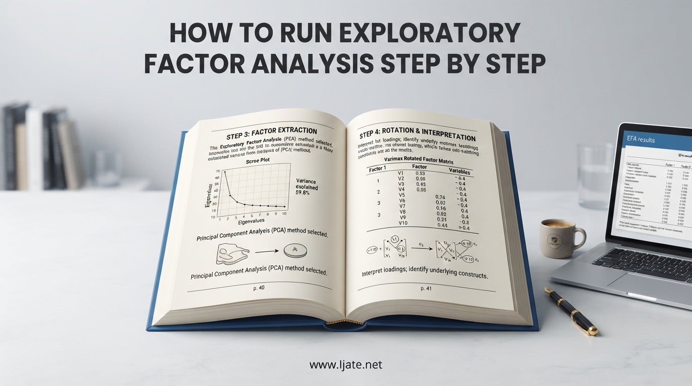
Learning how to run exploratory factor analysis step by step can feel overwhelming, especially if you are a graduate student staring at your first dataset with 30 survey items and no idea where to begin. I remember spending three weeks on a single EFA during my thesis, making every mistake in the book, and wishing someone had handed me a clear roadmap.
That is exactly what this guide is. I will walk you through every stage of exploratory factor analysis, from checking your correlation matrix to interpreting rotated factor loadings and writing up your results. Whether you use SPSS, R, or another statistical package, the same six-step workflow applies. Real researchers have applied this exact process in EFA in scale development studies, and you can too.
By the end of this article, you will know how to prepare your data, decide how many factors to extract, choose the right extraction and rotation methods, interpret your results with confidence, and avoid the common pitfalls that trip up most beginners. Let us get started.
Table of Contents
Quick Overview: The 6-Step EFA Workflow
Before diving into the details, here is the entire EFA process at a glance. Each step gets a full section later in this guide, but this overview helps you see the big picture.
Prepare your data and check assumptions – Screen for missing values, inspect the correlation matrix, and verify sampling adequacy with KMO and Bartlett’s test.
Determine the number of factors to extract – Use the Kaiser criterion, scree plot inspection, and parallel analysis to decide how many factors your data supports.
Choose an extraction method and extract factors – Select between principal components analysis, principal axis factoring, or maximum likelihood based on your research goals.
Rotate the factors – Apply Varimax (orthogonal) or Oblimin and Promax (oblique) rotation to achieve a simpler, more interpretable factor structure.
Interpret factor loadings and evaluate the solution – Examine the rotated factor matrix, check communalities, handle cross-loadings, and assess total variance explained.
Generate factor scores (optional) – Compute factor scores using the regression, Bartlett, or Anderson-Rubin method for use in subsequent analyses.
Think of these six steps as a cycle rather than a straight line. Researchers often loop back. You might extract three factors, rotate them, realize the solution does not make theoretical sense, and return to step two to try extracting two or four factors instead. That iterative process is completely normal.
Now let us break down each piece, starting with the fundamentals.
What Is Exploratory Factor Analysis?
Exploratory factor analysis (EFA) is a statistical technique used to identify the underlying structure of a set of observed variables by grouping them into a smaller number of latent factors that explain the correlations among them. In plain terms, EFA takes a large set of variables and figures out whether a few hidden constructs can explain the patterns in your data.
Imagine you have a 20-item personality questionnaire. EFA can tell you whether those 20 items actually measure three broader traits, like extraversion, conscientiousness, and emotional stability. The individual items are your observed variables. The traits they reflect are your latent variables, also called factors. This approach is widely used in EFA for identifying latent constructs across education, psychology, and social science research.
EFA serves two main purposes. First, it reduces data complexity by summarizing many variables into fewer factors. Second, it helps validate theoretical constructs by revealing whether your items cluster together the way you expected. This makes EFA a cornerstone of scale development and questionnaire validation.
Observed Variables vs. Latent Factors
The core idea behind factor analysis is that what we measure directly (observed variables) is influenced by things we cannot measure directly (latent factors). A survey item like “I feel nervous before exams” is an observed variable. The underlying anxiety construct it taps into is the latent factor.
EFA works backward from the observed data. It looks at how variables correlate and infers which latent factors might be causing those correlations. If two items correlate strongly, factor analysis assumes they share a common underlying cause.
Common Variance vs. Unique Variance
Every variable’s total variance can be split into three parts. Common variance is the portion shared with other variables through underlying factors. Specific variance is unique to that variable but is still reliable. Error variance is random measurement error.
Factor analysis focuses on common variance. This is what separates true factor analysis from principal components analysis, which analyzes all the variance in your data. Understanding this distinction matters when you choose an extraction method later in the process.
When to Use EFA
You should use exploratory factor analysis when you have a set of measured variables and want to discover the underlying factor structure without a strong pre-existing theory about how many factors exist or which variables load on them. EFA is exploratory by nature, meaning you let the data guide your understanding of the structure.
The most common scenario is scale development. If you created a new questionnaire with 30 items and want to know whether it measures two, three, or five distinct constructs, EFA is the right tool. Researchers routinely apply EFA in scale validation to confirm that their instruments behave as intended.
Other situations where EFA is appropriate include survey validation, where you want to check whether items group into expected dimensions, and data reduction, where you have too many variables and need to compress them into a manageable set of factors for further analysis. EFA is also useful when you are working with an existing instrument in a new population or language and want to verify that the factor structure still holds.
When NOT to Use EFA
Do not use EFA if you already have a strong, specific hypothesis about the exact factor structure and want to test it statistically. That is the job of confirmatory factor analysis (CFA). Using EFA when you should be using CFA is one of the most common mistakes researchers make.
Also avoid EFA if you have very few variables relative to the number of factors you expect, or if your sample size is too small. Both situations lead to unstable, unreplicable factor solutions.
EFA vs CFA vs PCA: Knowing the Difference
One of the biggest sources of confusion for researchers is the distinction between exploratory factor analysis (EFA), confirmatory factor analysis (CFA), and principal components analysis (PCA). These three techniques are related but serve different purposes and make different statistical assumptions.
EFA is used when you want to discover the factor structure in your data. CFA is used when you want to confirm a specific hypothesized structure. PCA is a data reduction technique that creates components from all the variance in your variables, not just the shared common variance that true factor analysis focuses on.
| Feature | EFA | CFA | PCA |
|---|---|---|---|
| Purpose | Discover factor structure | Test hypothesized structure | Reduce data dimensions |
| Variance analyzed | Common variance only | Common variance only | Total variance (common + specific + error) |
| Prior theory needed? | No | Yes | No |
| Latent constructs? | Yes | Yes | No (components are linear combinations) |
| Statistical test of fit? | Limited | Yes (chi-square, CFI, RMSEA, SRMR) | No |
| Typical use case | Scale development (early stage) | Scale validation (confirmatory) | Data compression, index creation |
The practical takeaway is this. Use EFA in the early stages of scale development when you are still exploring. Use CFA later with a new sample to confirm what EFA found. Use PCA only when your goal is purely data reduction and you are not interested in identifying latent constructs.
Many researchers on forums like Reddit’s r/statistics express frustration about this confusion. The most common complaint is running PCA in SPSS when they actually wanted to do EFA, because SPSS defaults to PCA under the Factor Analysis menu. This default trips up countless graduate students.
Key Concepts and Terminology
Before running EFA, you need to understand a handful of key terms. These concepts appear throughout every step of the analysis, so let me define them clearly.
Factor Loadings
A factor loading is the correlation between an observed variable and a latent factor. It tells you how strongly a particular item is associated with a given factor. Loadings range from -1 to +1, just like correlation coefficients.
The general rule of thumb for interpreting loadings is straightforward. Loadings of 0.30 or above are considered the minimum threshold for significance. Loadings of 0.40 are considered important, and loadings of 0.50 or above are considered strong. In practice, most researchers look for items loading at 0.40 or higher on their primary factor.
Eigenvalues
An eigenvalue represents the amount of variance in all the observed variables that a particular factor accounts for. A factor with an eigenvalue of 1.0 explains as much variance as a single original variable. This is the basis of the Kaiser criterion, which recommends retaining factors with eigenvalues greater than 1.0.
Higher eigenvalues mean the factor is explaining more of the total variance. The first factor always has the largest eigenvalue, and each subsequent factor explains less. This is why the first few factors are usually the most meaningful.
Communalities
Communality is the proportion of variance in an observed variable that is explained by all the extracted factors combined. It ranges from 0 to 1. A communality of 0.70 means that 70% of the variance in that variable is accounted for by the factor solution.
Low communalities (below 0.30 or 0.40) are a red flag. They suggest that the extracted factors do not explain much of the variance in that particular item. Items with consistently low communalities are candidates for removal from your scale.
Simple Structure
Simple structure is the goal of factor rotation. It means that each variable loads strongly on one factor and weakly on all others. When you achieve simple structure, interpretation becomes much easier because each factor represents a clear, distinct construct.
Thurstone first described the criteria for simple structure in 1947. The modern practical translation is that you want each item to have one high loading (above 0.40) and all other loadings should be substantially lower. Cross-loadings, where an item loads similarly on two or more factors, violate simple structure.
Cross-Loadings
A cross-loading occurs when a variable loads at a meaningful level (typically 0.32 or above) on two or more factors simultaneously. Cross-loadings make interpretation difficult because you cannot clearly assign the variable to a single factor.
Researchers handle cross-loadings in several ways. You can remove the cross-loading item entirely, which is the most common approach. You can also re-run the analysis with fewer factors or try a different rotation method. Some researchers keep the item if the difference between loadings is at least 0.15 and assign it to the factor where it loads highest.
Kaiser-Meyer-Olkin (KMO) Measure
The KMO measure of sampling adequacy tells you whether your data is suitable for factor analysis. It ranges from 0 to 1, with higher values indicating that patterns of correlation are relatively compact and factor analysis should yield distinct, reliable factors.
KMO values above 0.90 are considered excellent, 0.80 to 0.89 are good, 0.70 to 0.79 are acceptable, 0.60 to 0.69 are mediocre, and below 0.60 is unacceptable. If your overall KMO is below 0.60, you should seriously question whether factor analysis is appropriate for your data.
Bartlett’s Test of Sphericity
Bartlett’s test checks whether your correlation matrix is significantly different from an identity matrix, where all variables would be uncorrelated. A significant result (p less than 0.05) means that enough correlation exists among your variables to justify factor analysis.
If Bartlett’s test is not significant, your variables are essentially uncorrelated and factor analysis will not produce meaningful results. This test, combined with KMO, forms your initial data screening checkpoint before you proceed with extraction.
Prerequisites and Assumptions Before You Start
EFA makes several statistical assumptions about your data. Violating these assumptions can lead to misleading factor solutions, so it is worth checking each one before you begin the actual analysis.
Sample Size Requirements
Sample size is the most commonly asked question on statistics forums, and for good reason. EFA is a large-sample technique, and small samples produce unstable factor solutions that will not replicate.
The old rule of thumb was a minimum ratio of 5 to 10 participants per variable. So if you have 30 items, you would need 150 to 300 participants. However, modern research has shown that this ratio alone is insufficient.
A more reliable guideline comes from MacCallum and colleagues, who recommend absolute sample sizes based on communalities. If your communalities are high (above 0.60) and factors are well-determined (four or more strong loadings per factor), even 100 to 200 participants can work. With moderate communalities (0.40 to 0.60), aim for 200 to 400. With lower communalities, you may need 500 or more.
As a practical minimum, most methodologists agree that N = 150 is the floor for EFA. For a 20-item scale, 200 to 300 participants is a reasonable target. When in doubt, collect more data.
Level of Measurement
Traditional EFA assumes continuous, interval-level data with a multivariate normal distribution. In practice, most researchers apply EFA to Likert-scale items rated on 5-point or 7-point scales. While this technically violates the interval assumption, EFA tends to be robust to this violation with 5 or more response options.
For binary or 3-point scales, consider alternatives like tetrachoric or polychoric correlation matrices instead of Pearson correlations. In R, the psych package handles this automatically. In SPSS, you would need additional procedures.
Linearity and Normality
EFA assumes linear relationships among variables. If your correlations are curvilinear, factor analysis may miss important patterns. You can check this by examining scatterplot matrices.
While maximum likelihood extraction assumes multivariate normality, principal axis factoring and principal components analysis do not require it. This is one reason many researchers default to PAF when normality is questionable.
No Extreme Multicollinearity
If two variables are extremely highly correlated (above 0.90), they are essentially measuring the same thing. This can cause computational problems in factor analysis. Check your correlation matrix for any pairs of variables with correlations above 0.85 and consider combining or removing one of them.
Adequate Correlations Among Variables
For EFA to work, there must be meaningful correlations among your variables. If most correlations in your matrix are below 0.30, factor analysis may not reveal meaningful factors. The KMO measure and Bartlett’s test formally check this assumption, which brings us to step one of the actual analysis.
How to Run Exploratory Factor Analysis Step by Step
Now we get to the heart of this guide. Here is the detailed, step-by-step process of running exploratory factor analysis. I will cover each of the six steps introduced in the quick overview, with specific instructions for SPSS and R along the way.
These six steps represent the complete EFA workflow. Follow them in order, but remember that you will likely cycle back as you refine your solution.
Step 1: Prepare Your Data and Check Assumptions
The first step is to prepare your dataset and verify that it meets the assumptions for factor analysis. Skipping this step is the most common reason that EFA produces nonsense results.
1.1 Screen for Missing Data
Start by examining your dataset for missing values. Most EFA procedures use listwise or pairwise deletion, meaning rows with missing data get dropped. If you have a lot of missing data, you may lose a significant portion of your sample.
Check the percentage of missing data per variable and per case. If a variable has more than 5% missing values, investigate why. If a participant has missing data on more than 20% of items, consider excluding them entirely.
For small amounts of missing data, mean substitution or expectation-maximization (EM) imputation can work. For larger amounts, multiple imputation is the gold standard. In SPSS, you can use the Missing Value Analysis module. In R, the mice package is widely used.
1.2 Examine the Correlation Matrix
Before running factor analysis, look at your correlation matrix. You want to see a healthy number of correlations above 0.30. If most correlations are near zero, your variables may not share enough common variance for factors to emerge.
Watch for the opposite problem too. If almost all correlations are above 0.80, your variables may be too similar and you might end up with a single dominant factor. A good correlation matrix has a mix of moderate correlations with some variables correlating more strongly in subgroups.
1.3 Run the KMO Test
The Kaiser-Meyer-Olkin measure tells you whether sampling adequacy is sufficient. Run it before extraction. In SPSS, go to Analyze, then Dimension Reduction, then Factor, click on Descriptives, and check KMO and Bartlett’s test of sphericity.
In R, you can use the KMO function from the psych package. The command is KMO(yourdata). This returns both the overall KMO and the KMO for each individual variable.
If your overall KMO is below 0.60, consider removing variables with the lowest individual KMO values and re-running the test. This can sometimes push the overall KMO above the threshold.
1.4 Run Bartlett’s Test of Sphericity
Bartlett’s test appears in the same SPSS dialog as KMO. It tests whether your correlation matrix is significantly different from an identity matrix. You want a significant result, meaning p less than 0.05.
If Bartlett’s test is not significant, your variables do not correlate enough for factor analysis. This usually means you need different variables or a different research question. No amount of rotation or extraction method changes will fix fundamentally uncorrelated data.
1.5 Check for Outliers
Extreme outliers can distort correlations and, by extension, your factor solution. Run a quick check for multivariate outliers using Mahalanobis distance or Cook’s distance. Remove or correct extreme cases before proceeding.
1.6 Decision Checkpoint
Before moving to step two, confirm the following. KMO is above 0.60, Bartlett’s test is significant, most correlations are above 0.30, no extreme multicollinearity exists, and your sample size is adequate. If all boxes are checked, you are ready to determine the number of factors.
Step 2: Determine the Number of Factors to Extract
Deciding how many factors to retain is one of the most consequential decisions in the entire EFA process. Extract too few factors and you merge distinct constructs. Extract too many and you split a single construct into meaningless fragments.
There is no single correct method for this decision. The best approach is to use multiple criteria, compare their recommendations, and make an informed judgment guided by theory.
2.1 Kaiser Criterion (Eigenvalues Greater Than 1)
The Kaiser criterion, also called the Guttman-Kaiser rule or the root-one criterion, retains any factor with an eigenvalue greater than 1.0. The logic is that a factor should explain at least as much variance as a single original variable to be worth keeping.
This is the default method in SPSS, which is both convenient and dangerous. The Kaiser criterion tends to over-extract factors, especially with many variables. It is a useful starting point but should never be your only criterion.
2.2 Scree Plot Inspection
A scree plot graphs eigenvalues from largest to smallest. You look for the “elbow” or point where the curve levels off. The classic approach, proposed by Cattell in 1966, is to retain all factors above the elbow point.
Reading scree plots requires judgment. The elbow is not always obvious. Some researchers advocate retaining factors up to and including the one at the elbow, while others say to stop just before it. When the plot is ambiguous, parallel analysis provides a more objective answer.
In SPSS, the scree plot is generated automatically when you check the option in the Extraction dialog. In R, the psych package provides scree plots with the scree(yourdata) or fa.parallel(yourdata) commands.
2.3 Parallel Analysis
Parallel analysis is currently considered the most accurate method for determining the number of factors. It works by generating random datasets with the same number of variables and participants as your actual data, computing eigenvalues for those random datasets, and comparing them to your real eigenvalues.
You retain factors whose eigenvalues exceed the corresponding eigenvalues from the random data. This method accounts for chance variation and significantly reduces the over-extraction problem of the Kaiser criterion.
In R, run parallel analysis with fa.parallel(yourdata, fa = "fa") from the psych package. The function generates the plot and tells you exactly how many factors to retain. In SPSS, parallel analysis requires custom syntax or an external tool, which is one reason many researchers switch to R for EFA.
2.4 Minimum Average Partial (MAP) Test
The MAP test, developed by Velicer, is another objective method for determining the number of factors. It examines the average partial correlation after extracting successive factors. The number of factors that produces the lowest average partial correlation is the recommended solution.
The MAP test is available in R through the psych package using VSS(yourdata). Some researchers prefer MAP over parallel analysis for factors with strong loadings, while parallel analysis performs better with weaker loadings.
2.5 Theoretical Judgment
After consulting Kaiser, scree plots, parallel analysis, and MAP, the final decision should be guided by theory. If parallel analysis says three factors but your theoretical framework predicts four, try both solutions and compare interpretability.
The best factor solution is one that is both statistically supported and theoretically meaningful. A clean three-factor solution that makes conceptual sense is always better than a messy five-factor solution just because Kaiser says five.
Step 3: Choose an Extraction Method and Extract Factors
Factor extraction is the mathematical process of deriving initial factors from your correlation matrix. Several extraction methods exist, and your choice depends on your data characteristics and research goals.
3.1 Principal Components Analysis (PCA)
PCA analyzes all the variance in your variables, not just common variance. It creates linear combinations of the original variables called components. PCA is technically a data reduction technique rather than a true factor analysis method.
Use PCA when your goal is purely data reduction and you do not need to identify latent constructs. PCA is also the default in SPSS under the Factor Analysis menu, which is why so many researchers accidentally run it when they mean to do EFA.
3.2 Principal Axis Factoring (PAF)
Principal axis factoring, also called common factor analysis, analyzes only the shared variance among variables. It uses squared multiple correlations as initial communality estimates and iteratively refines them.
PAF does not require multivariate normality, making it a good choice for non-normal data. It is the recommended default for most exploratory factor analyses where the goal is to identify latent constructs. In SPSS, select Principal axis factoring from the Method dropdown in the Extraction dialog.
3.3 Maximum Likelihood (ML)
Maximum likelihood estimation is a model-based extraction method that assumes multivariate normality. Its major advantage is that it provides goodness-of-fit statistics and confidence intervals for factor loadings, which PAF cannot do.
Use ML when your data is approximately normal and you want statistical tests of model fit. ML also allows you to compare different factor solutions using chi-square difference tests. However, ML is sensitive to violations of normality and can produce poor results with non-normal data.
3.4 Comparison of Extraction Methods
| Criterion | PCA | PAF | Maximum Likelihood |
|---|---|---|---|
| Variance analyzed | Total variance | Common variance | Common variance |
| Normality assumed? | No | No | Yes |
| Goodness-of-fit test? | No | No | Yes |
| Identifies latent constructs? | No | Yes | Yes |
| Best for | Data reduction | General EFA | Normal data, model comparison |
For most applied research situations, principal axis factoring is the safest choice. It does not require normality, focuses on common variance, and produces results very similar to maximum likelihood when assumptions are met. If you need fit statistics and your data is normal, switch to maximum likelihood.
Step 4: Rotate the Factors
Initial factor extraction produces a mathematically correct but practically useless solution. The initial factors are usually correlated with most variables at moderate levels, making interpretation nearly impossible. Rotation solves this problem by redistributing the variance to achieve a simpler, more interpretable structure.
Rotation does not change how much variance the factor solution explains. It only changes the perspective from which you view that variance. Think of it as rotating a 3D object to find the angle where its features are most clearly visible.
4.1 Orthogonal Rotation
Orthogonal rotations assume that the underlying factors are uncorrelated with each other. The most common orthogonal rotation is Varimax, which maximizes the variance of squared loadings within each factor. Varimax tries to push high loadings higher and low loadings lower, making the structure easier to interpret.
Other orthogonal options include Quartimax, which tends to produce a strong general factor, and Equamax, which is a compromise between Varimax and Quartimax. In practice, Varimax is the most widely used orthogonal rotation and the default in most software.
Choose orthogonal rotation only if you have a strong theoretical reason to believe your factors are independent. In social science research, most psychological constructs are correlated, making this assumption unrealistic.
4.2 Oblique Rotation
Oblique rotations allow the underlying factors to correlate with each other. This is more realistic for most social science and education research, where constructs like anxiety and depression naturally overlap.
The most common oblique rotations are Direct Oblimin and Promax. Direct Oblimin has a parameter called delta that controls how much factors are allowed to correlate. A delta of 0 allows moderate correlations. A negative delta restricts correlations more, while a positive delta allows higher correlations.
Promax is computationally faster and is often preferred for large datasets. It works by first performing an orthogonal Varimax rotation and then raising the loadings to a power (the kappa parameter) to simplify the structure. A kappa of 4 is the default in most software.
4.3 Comparison of Rotation Methods
| Rotation | Type | Factors Correlated? | Best For |
|---|---|---|---|
| Varimax | Orthogonal | No (assumed independent) | Uncorrelated theoretical constructs |
| Quartimax | Orthogonal | No | When a general factor is expected |
| Equamax | Orthogonal | No | Compromise between Varimax and Quartimax |
| Direct Oblimin | Oblique | Yes | Realistic social science constructs |
| Promax | Oblique | Yes | Large datasets, faster computation |
4.4 Which Rotation Should You Choose?
The current consensus among methodologists, including Fabrigar, Wegener, MacCallum, and Strahan in their influential 1999 paper, is to default to oblique rotation. If the factors turn out to be uncorrelated, oblique rotation will show near-zero correlations and you lose nothing. If the factors are truly correlated, only oblique rotation will reveal the true structure.
After running an oblique rotation, always check the factor correlation matrix. If factor correlations are below 0.30, orthogonal and oblique solutions will be nearly identical, and either is acceptable. If correlations exceed 0.50, oblique rotation was clearly necessary.
In SPSS, select Direct Oblimin from the Rotation dialog and leave delta at 0. In R, the psych package makes it easy with fa(yourdata, nfactors = 3, rotate = "oblimin").
4.5 Pattern Matrix vs. Structure Matrix
With oblique rotation, you get two matrices instead of one. The pattern matrix shows the unique contribution of each variable to each factor, controlling for other factors. The structure matrix shows the total correlation between each variable and each factor, including indirect effects through factor correlations.
For interpreting which items belong to which factor, use the pattern matrix. It gives you the cleanest picture of unique factor-variable relationships. The structure matrix can inflate apparent loadings because it includes the shared variance between correlated factors.
This is a subtle but important point. Reporting the wrong matrix can mislead readers about the strength of your factor solution. Always specify which matrix you are interpreting.
Step 5: Interpret Factor Loadings and Evaluate the Solution
After extraction and rotation, you are ready to interpret your results. This step requires both statistical judgment and theoretical understanding. The numbers alone do not tell the full story.
5.1 Examine the Rotated Factor Matrix
Start by looking at the pattern matrix (if you used oblique rotation) or the rotated component matrix (if you used Varimax). For each factor, identify which variables load at 0.40 or above. These are the items that define the factor.
Give each factor a name based on the content of its highest-loading items. If items about nervousness, worry, and tension load together on factor one, you might name it “Anxiety.” This naming process forces you to think about what each factor represents conceptually.
5.2 Check Factor Loading Thresholds
Use these established thresholds for interpreting loadings. A loading of 0.32 explains approximately 10% of the overlap between the variable and the factor, which many consider the minimum for practical significance. A loading of 0.45 explains about 20%, and 0.55 explains about 30%.
In practice, look for items with loadings above 0.40 on their primary factor. If an item loads below 0.32 on all factors, it is not measuring any of the identified constructs well and should be removed.
5.3 Handle Cross-Loadings
Cross-loadings occur when a variable loads at 0.32 or above on two or more factors. They are one of the most frustrating problems in EFA because they make interpretation ambiguous.
Here is how I recommend handling cross-loadings, based on the common experiences researchers share on statistics forums. First, check whether the difference between the primary and secondary loading is at least 0.15. If so, you can reasonably assign the item to its primary factor.
If the loadings are similar across factors, try removing the item and re-running the analysis. Often, one problematic item causes multiple cross-loadings, and removing it cleans up the entire solution. If cross-loadings persist across many items, you may need to extract a different number of factors or try a different rotation method.
5.4 Evaluate Communalities
Check the communalities table for each variable. Most communalities should be above 0.40, and ideally above 0.50. Items with communalities below 0.30 are poorly explained by the factor solution and should be considered for removal.
Low communalities across many items suggest that your extraction method or number of factors may need adjustment. If you used PCA, switching to PAF can sometimes improve communalities because PAF focuses specifically on shared variance.
5.5 Assess Total Variance Explained
Look at the total variance explained table. For social science research, a three to five factor solution explaining 50% to 75% of the total variance is generally acceptable. Higher is always better, but do not sacrifice interpretability for a few extra percentage points of variance.
The cumulative variance explained depends on your field. In personality research, solutions explaining 40% to 50% of variance are common because human behavior is complex. In more structured domains like aptitude testing, you might expect 70% or more.
5.6 Iterative Refinement
EFA is almost always iterative. After your first run, you will likely identify items to remove, a different number of factors to try, or a different rotation to test. Remove one item at a time, re-run the analysis, and check how the solution changes.
Document each decision. When you write up your results, reviewers and committee members will want to know not just your final solution but the path you took to get there. Keeping a log of which items you removed and why makes this reporting straightforward and supports related measurement analysis transparency.
5.7 Reproducibility Check
If possible, split your sample and run EFA on each half separately. If the same factor structure emerges in both halves, you have strong evidence for the stability of your solution. This split-sample approach is one of the simplest forms of cross-validation available.
Step 6: Generate Factor Scores (Optional)
After interpreting your factor solution, you may want to compute factor scores for each participant. These scores represent each person’s standing on the latent factors and can be used in subsequent analyses like regression, group comparisons, or correlations with external variables.
6.1 Why Generate Factor Scores?
Factor scores collapse multiple items into a single composite score per factor per participant. This dramatically simplifies downstream analyses. Instead of running a regression with 20 individual items, you run it with 3 factor scores.
Factor scores are also useful for creating a total scale score. If your EFA confirms that all items load on a single factor, the factor score is the most statistically sound way to combine them.
6.2 Factor Score Methods Compared
| Method | Characteristics | Best For |
|---|---|---|
| Regression | Most common, can produce correlated scores even with orthogonal rotation | General use, produces scores with highest correlation to true factor |
| Bartlett | Minimizes mean squared error, produces unbiased scores | When unbiased estimation is prioritized |
| Anderson-Rubin | Produces uncorrelated scores even with oblique factors, standardized to mean 0 and SD 1 | When uncorrelated scores are required for downstream analysis |
In SPSS, select the Regression method under the Scores button in the Factor Analysis dialog. New variables will appear at the end of your dataset labeled FAC1_1, FAC2_1, and so on. In R, the psych package saves factor scores when you use the fa() function with the scores = "regression" argument.
6.3 Simple Alternatives
If you do not need the statistical precision of computed factor scores, a simpler alternative is to average or sum the items that load on each factor. This creates unit-weighted composite scores that are easy to compute, easy to explain, and often perform similarly to regression-based factor scores in practical applications.
Many researchers prefer this approach for reporting purposes because it is transparent and reproducible. Factor scores, by contrast, depend on weights that change with every new sample.
How to Report EFA Results in APA Format
Reporting EFA results clearly and completely is essential for thesis, dissertation, and journal article writing. Yet no major competitor in the SERP covers this topic, leaving researchers to figure it out on their own. Here is what to include.
Describe Your Analytical Decisions
Start by stating the extraction method, rotation method, and how you determined the number of factors. For example, write that you used principal axis factoring with Direct Oblimin rotation and that parallel analysis indicated a three-factor solution. This transparency helps readers evaluate the quality of your analysis.
Also report your sample size, the number of items analyzed, and the ratio of participants to variables. Reviewers in psychometrics and education research expect this information.
Report Data Screening Results
State the KMO value and Bartlett’s test result. For example, write that KMO was 0.82, indicating good sampling adequacy, and Bartlett’s test of sphericity was significant, chi-squared equals 1247.3, df equals 136, p is less than 0.001. This shows that your data was suitable for factor analysis.
Present the Factor Matrix
Include a table showing the pattern matrix (for oblique rotation) or rotated factor matrix (for orthogonal rotation). Show all factor loadings above 0.30 or 0.32. Bold or underline the primary loadings for each item. Also include communalities for each variable.
If you used oblique rotation, report the factor correlation matrix as well. This lets readers see how strongly your factors are related to each other.
Report Variance Explained
State the eigenvalues for each retained factor and the percentage of variance each factor explains. Report the cumulative variance explained by all retained factors together. For example, write that the three factors explained 58.3% of the total variance collectively.
Name and Interpret Each Factor
For each factor, describe the items that load on it and explain the conceptual meaning you assigned. Connect the factor names back to your theoretical framework. This interpretive section is where you demonstrate that your factor solution makes theoretical sense.
Sample APA Write-Up
Here is a condensed example of how an EFA write-up might look in APA format:
“To examine the factor structure of the 20-item scale, we conducted an exploratory factor analysis using principal axis factoring with Direct Oblimin rotation (delta = 0). Prior to analysis, we assessed the suitability of the data for factor analysis. The KMO measure of sampling adequacy was 0.84, exceeding the recommended threshold of 0.60. Bartlett’s test of sphericity was significant, chi-squared (190) = 1542.67, p is less than 0.001. Parallel analysis suggested a three-factor solution. The three factors collectively accounted for 54.2% of the variance. All items loaded above 0.40 on their primary factor, with no significant cross-loadings. Factor correlations ranged from 0.24 to 0.41.”
Common Mistakes to Avoid When Running EFA
After reviewing hundreds of forum posts from frustrated graduate students and researchers, I have identified the most common mistakes that derail EFA. Avoid these and you will save yourself weeks of frustration.
Mistake 1: Confusing PCA with EFA
This is the number one mistake, and it is not entirely the researcher’s fault. SPSS defaults to principal components analysis under the Factor Analysis menu, and many users never realize they are running the wrong procedure. PCA analyzes total variance while EFA analyzes common variance. They can produce similar results, but they answer different questions.
If your goal is to identify latent constructs, explicitly change the extraction method from PCA to principal axis factoring or maximum likelihood. This single change often resolves mysterious discrepancies between your results and published EFA examples.
Mistake 2: Relying Solely on the Kaiser Criterion
The Kaiser criterion, retaining factors with eigenvalues above 1.0, is the default in most software but is known to over-extract. It is particularly problematic with 30 or more variables. Always supplement Kaiser with parallel analysis or MAP testing for a more accurate factor count.
Mistake 3: Defaulting to Varimax Without Thinking
Varimax is the SPSS default rotation, but it forces factors to be uncorrelated. In most social science applications, constructs are naturally correlated. Using Varimax when factors are actually related can distort the factor structure and produce misleading results.
Always start with an oblique rotation like Direct Oblimin. Check the factor correlation matrix. If correlations are near zero, you can switch to Varimax for a cleaner presentation. If correlations are substantial, oblique rotation was the right call.
Mistake 4: Over-Extracting Factors
Extracting too many factors splits a single construct into meaningless fragments. You might see a factor with only one or two items loading on it, which is almost never a stable, replicable factor. If a factor has fewer than three items with loadings above 0.40, consider reducing the number of factors.
Mistake 5: Ignoring Cross-Loadings
Cross-loadings do not go away just because you do not report them. If an item loads at 0.42 on factor one and 0.38 on factor two, that is a cross-loading that needs to be addressed. Removing cross-loading items improves clarity and replicability of your factor solution.
Mistake 6: Deleting Items Without Justification
It is tempting to delete items until you get a clean factor structure. But every deletion should be justified statistically and theoretically. If you delete ten items from a 20-item scale, reviewers will question whether your scale was well-designed in the first place. Document your reasoning for each deletion.
Mistake 7: Not Checking Communalities
Low communalities indicate that the factor solution does not explain much variance for those items. Ignoring low communalities and reporting the solution anyway hides a weakness in your analysis. Check communalities, remove items with values below 0.30, and re-run.
Mistake 8: Small Sample Sizes
Running EFA with 50 participants on a 20-item scale produces results that will never replicate. If your sample is too small, collect more data. No analytical trick compensates for insufficient data.
Mistake 9: Not Reading the Pattern Matrix for Oblique Solutions
When using oblique rotation, some researchers accidentally report the structure matrix instead of the pattern matrix. The structure matrix inflates loadings because it includes indirect correlations through factor relationships. Always interpret and report the pattern matrix for oblique rotations.
Mistake 10: Treating EFA Results as Final
EFA is exploratory. Its results suggest a structure that needs confirmation with new data. Running CFA on the same sample that produced the EFA is circular and inflates fit statistics. Always validate your EFA-derived structure with CFA on an independent sample.
FAQs
How to interpret exploratory factor analysis results?
To interpret EFA results, examine the rotated pattern matrix and identify which variables load at 0.40 or above on each factor. Name each factor based on the content of its highest-loading items. Check communalities (aim for 0.40 or above per item), review the total variance explained (50% or more is typical in social science), and examine the factor correlation matrix if you used oblique rotation. Remove items with low loadings or problematic cross-loadings, then re-run the analysis to confirm the refined structure is stable and theoretically meaningful.
What is the main purpose of exploratory factor analysis?
The main purpose of exploratory factor analysis is to identify the underlying latent factor structure in a set of observed variables. EFA groups correlated variables together into factors, reducing data complexity by summarizing many measured items into fewer unobserved constructs. It is primarily used in scale development, questionnaire validation, and data reduction to discover how many distinct dimensions a set of variables measures and which items belong to each dimension.
What’s the difference between EFA and CFA?
EFA is exploratory and lets the data reveal the factor structure without a pre-specified hypothesis, while CFA is confirmatory and tests whether a specific hypothesized factor structure fits the data. EFA allows all variables to load on all factors, estimates the number of factors from the data, and provides limited fit statistics. CFA requires you to specify which variables load on which factors beforehand, restricts cross-loadings to zero, and provides comprehensive goodness-of-fit indices like CFI, RMSEA, and SRMR. EFA is used early in scale development; CFA is used later to validate the structure with new data.
How to conduct EFA in SPSS?
To conduct EFA in SPSS, go to Analyze, then Dimension Reduction, then Factor. Move your variables into the analysis box. Under Descriptives, check KMO and Bartlett’s test of sphericity. Under Extraction, change the method from PCA to Principal Axis Factoring, and select Scree plot. Under Rotation, select Direct Oblimin. Under Scores, check Save as variables and select Regression if you want factor scores. Click OK to run. Review the KMO value (above 0.60), check the scree plot and eigenvalues for the number of factors, and interpret the pattern matrix for loadings above 0.40.
Conclusion
Learning how to run exploratory factor analysis step by step takes practice, but the six-step framework in this guide gives you a reliable roadmap. Prepare your data and verify assumptions with KMO and Bartlett’s test. Determine the number of factors using parallel analysis rather than relying on Kaiser alone. Extract with principal axis factoring unless you have a specific reason to choose otherwise. Rotate with an oblique method like Direct Oblimin. Interpret the pattern matrix carefully, handling cross-loadings and checking communalities. Optionally generate factor scores for downstream analysis.
The most important thing to remember is that EFA is iterative. You will rarely get your final solution on the first run. Be patient, document every decision, and let theory guide your interpretation alongside statistics. Once you have a stable factor solution, the natural next step is to confirm it with an independent sample using confirmatory factor analysis (CFA) follow-up.