Guide to Deciding Factor Retention in Exploratory Factor Analysis in (2026)

Deciding how many factors to retain in exploratory factor analysis (EFA) is one of the most consequential and frequently debated decisions in psychometric research. Get it right and your measurement model reflects genuine latent constructs that hold up across samples and studies. Get it wrong and you either force artificial dimensions onto your data or collapse distinct constructs into muddy, uninterpretable factors that undermine everything downstream of your analysis. Researchers across psychology, education, health sciences, and the broader social sciences rely on this decision every time they build a questionnaire, validate an instrument, or explore the dimensional structure of a new construct.

If you have ever run EFA in SPSS or R and watched the Kaiser criterion, the scree plot, parallel analysis, and the Velicer MAP test each return a different number of factors, you already know how frustrating this decision can be. One Reddit user captured the experience perfectly when they wrote, “I hate exploratory factor analysis… every step is subjective… the eigenvalue criterion – almost half of the literature accepts this and half rejects it.” That confusion is exactly what this guide addresses.

Our team has spent years running EFA on scale development projects, and we have read through hundreds of forum threads on Reddit, ResearchGate, and CrossValidated to understand where researchers get stuck. In this article you will learn every major method for deciding the number of factors to retain, when to trust each one, and most importantly how to decide the number of factors to retain in exploratory factor analysis when multiple methods disagree. We also cover emerging methods like Exploratory Graph Analysis and provide a step-by-step decision framework you can apply to your own data today.

This guide is written for researchers, graduate students, and practitioners who need to make defensible factor retention decisions in published work. Whether you are working on scale development, questionnaire validation, or a broader psychometric assessment, the methods and framework below will help you report your decisions with confidence and survive peer review.

The Quick Answer: Best Practices for Factor Retention in 2026

If you need the short version before diving into the full guide, here it is. The current consensus in the methodological literature, supported by simulation studies from Auerswald and Moshagen (2019) and Ruscio and Roche (2012), is that parallel analysis is the most accurate single method for deciding the number of factors to retain in EFA. The Kaiser eigenvalue-greater-than-one criterion is widely considered outdated and prone to over-extraction, though it remains the default in SPSS and many other statistical packages.

The best practice is to run multiple methods and look for convergence. At minimum, run parallel analysis, examine the scree plot, and compute the Velicer MAP test. If two or more of these methods agree, you have a defensible answer that you can justify to reviewers. If they disagree, default to parallel analysis but also consider theoretical interpretability, the simplicity of your factor structure, and whether each retained factor has at least three to four variables loading at 0.40 or higher.

We explain the reasoning behind each recommendation in detail below, including how to handle the most common conflict scenarios that researchers report on forums. We also cover less common methods like Very Simple Structure, Exploratory Graph Analysis, and Bayesian approaches so that you have a complete picture of every tool available to you.

Overview of Factor Retention Methods

Before we walk through each method individually, here is a side-by-side overview of every major factor retention criterion. No single competitor in the search landscape provides this complete comparison, so we built it from the simulation literature and forum discussions to give you the full map at a glance.

The methods fall into three tiers based on their accuracy in Monte Carlo simulation studies. Tier one methods, including parallel analysis and the Velicer MAP test, show the highest accuracy rates across sample sizes and factor structures. These are the methods you should rely on most heavily. Tier two methods, including the scree plot and Very Simple Structure, are useful as confirmatory evidence but should not be the sole basis for your decision. Tier three methods, including the Kaiser eigenvalue criterion, are the most widely used in practice but also the most criticized in the contemporary methodological literature.

Parallel analysis. Compares your real eigenvalues to eigenvalues from random data of the same size. You retain factors whose eigenvalues exceed the random-data benchmark. This method is the top recommendation of methodological reviewers and performs best in head-to-head simulations.

Velicer MAP test. Minimizes the average partial correlation after each factor is extracted. The number of factors at the minimum MAP value is your answer. Particularly strong for identifying smaller factors that other methods might miss.

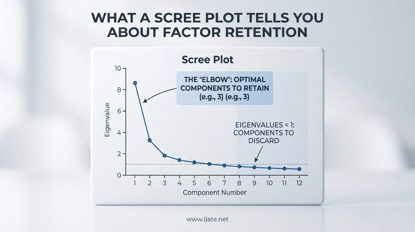
Scree plot (Cattell’s test). You plot eigenvalues in descending order and look for the point where the curve levels off. The factors above the elbow are retained. Subjective but useful as a visual check against the other methods.

Kaiser criterion (eigenvalue greater than one). Retain any factor with an eigenvalue above 1.0. Simple, automated, and over-extracts. Originally developed for PCA, not EFA, but still the SPSS default.

Very Simple Structure (VSS). Evaluates how well each factor solution approximates a simple structure where each variable loads on only one factor. Reports a complexity value from one upward and identifies the solution with the cleanest structure.

Exploratory Graph Analysis (EGA). A newer method that uses network estimation and community detection algorithms to identify the number of factors. Increasingly cited in the recent literature and available through the EGAnet R package.

Bayesian approaches. Emerging methods that use posterior probabilities and model comparison indices like BIC, WAIC, and deviance information criteria to compare factor solutions. Computationally intensive but promising.

Theoretical and interpretability checks. Not a statistical method on its own, but the final arbiter. Every retained factor must be theoretically meaningful, interpretable, and supported by at least three substantive loadings. If the statistics and the theory conflict, you need to understand why before proceeding.

The Eigenvalue Criterion (Kaiser Method)

The Kaiser criterion, also known as the eigenvalue-greater-than-one rule or the Kaiser-Guttman rule, is the oldest and most widely used default for deciding the number of factors to retain. The rule is simple: any factor with an eigenvalue above 1.0 is retained, and any factor with an eigenvalue below 1.0 is dropped. SPSS applies this criterion by default in its factor analysis dialog, which is one reason it remains so prevalent despite decades of criticism in the methodological literature.

The logic behind the rule is that an eigenvalue of 1.0 means the factor explains as much variance as a single original variable. If a factor explains less variance than one variable, the argument goes, it is not pulling its weight and should be dropped. On the surface this seems reasonable, and it has the appeal of being completely objective with no judgment calls required.

The problem is that the Kaiser criterion was originally developed for principal components analysis, not common factor analysis. In PCA every variable contributes a full unit of variance and the total is exactly equal to the number of variables, so an eigenvalue of 1.0 is a meaningful midpoint. In common factor analysis the variance being analyzed is the shared variance only, and the cutoff of 1.0 has no equivalent mathematical meaning. The criterion also ignores sampling variability, treating each eigenvalue as if it were measured without error.

Simulation studies have consistently shown that the Kaiser criterion over-extracts factors. It tends to retain one or two extra factors beyond the true structure, especially with larger variable sets and smaller sample sizes. A researcher on CrossValidated noted that the eigenvalue criterion “almost half of the literature accepts this and half rejects it,” which fairly captures the divide. The classical scale development literature from the 1970s and 1980s relied heavily on it, while contemporary methodological guidance from Preacher and MacCallum (2003) onward recommends against using it as a sole criterion.

In practice, the Kaiser criterion tends to produce factor solutions where the last one or two factors have very few substantive loadings and are not theoretically interpretable. If you find yourself trying to name a factor that has only one or two variables loading above 0.40, you may well be looking at the over-extraction that the Kaiser criterion is known for.

Our recommendation: report the Kaiser criterion result for completeness and because reviewers may ask about it, but never let it be the deciding factor in your retention decision. Treat it as a maximum ceiling on the number of factors rather than a target. If Kaiser says five factors and parallel analysis says three, the answer is almost certainly three.

The Scree Plot (Cattell’s Scree Test)

The scree plot, introduced by Raymond Cattell in 1966, is a visual method for deciding the number of factors to retain. You plot the eigenvalues of all possible factors in descending order and look for the point where the steep decline flattens out into a gentle tail. The factors before the elbow are retained and the factors along the tail are dropped. The name comes from the geological term scree, which refers to the rubble that accumulates at the base of a cliff.

Reading a scree plot sounds straightforward until you actually try it. The elbow is often ambiguous, and different researchers looking at the same plot routinely identify different cutoff points. A Reddit user posted a scree plot and asked “Where is the elbow??” – a question that every researcher who has run EFA has asked at some point. The honest answer is that scree plot interpretation requires judgment and benefits from practice with datasets where the true structure is known.

Here is a practical approach. First, look at where the curve transitions from a steep drop to a relatively flat slope. Then, identify the last point on the steep portion before the leveling begins. You retain all factors up to and including that point, but not the factor at which the leveling begins. If you see a sharp drop from eigenvalue 3.2 to 1.4 to 0.9 to 0.7, the elbow is at the transition between 1.4 and 0.9, and you retain two factors.

Some methodologists recommend an alternative approach called the smooth scree or the optimal coordinates method, which fits lines to the eigenvalue curve and identifies the breakpoint algorithmically. This removes some of the subjectivity but is less widely used and not available in standard software without additional programming.

The scree plot works best when the factor structure is clear and the eigenvalues show a dramatic drop followed by a long flat tail. It struggles when the eigenvalues decline gradually without a clear break, when there are many small factors, or when sample size is small enough that the eigenvalues are noisy and the curve is rough rather than smooth.

Our recommendation: always generate and examine the scree plot because reviewers expect to see it and because it can sometimes reveal factor structures that eigenvalue-based methods miss. Use it as confirmatory evidence alongside parallel analysis rather than as the primary basis for your decision. If the scree plot agrees with parallel analysis you have a strong case. If it disagrees, prefer parallel analysis and explain the discrepancy in your write-up with reference to the subjectivity of visual interpretation.

Parallel Analysis: The Recommended Method

Parallel analysis is widely regarded as the most accurate method for deciding the number of factors to retain in exploratory factor analysis. The method was introduced by Horn in 1965 and has been validated extensively through Monte Carlo simulation studies, including the influential Ruscio and Roche (2012) paper cited over 781 times in the academic literature and the comprehensive comparison by Auerswald and Moshagen (2019) in Psychological Methods.

Here is how parallel analysis works. The procedure generates a large number of random datasets, each with the same number of variables and the same sample size as your real dataset, but with values drawn from a normal distribution where no underlying factor structure exists. For each random dataset, eigenvalues are computed and stored. The result is a distribution of random eigenvalues against which your real eigenvalues can be compared.

You retain only the factors whose real-data eigenvalues exceed the corresponding random-data eigenvalues at a chosen percentile, typically the 95th percentile. The logic is that a factor only counts as meaningful if it explains more variance than you would expect from pure noise. Factors that do not beat the random benchmark are treated as noise and dropped from the analysis.

The reason parallel analysis outperforms simpler methods is that it accounts for sampling variability. The Kaiser criterion treats each eigenvalue as a fixed value, but in reality eigenvalues fluctuate from sample to sample. By comparing against a distribution of eigenvalues from random data, parallel analysis builds in a correction for the fact that some factors will look meaningful by chance alone.

In R, you can run parallel analysis through the psych package using the fa.parallel function. A typical call looks like fa.parallel(yourdata, fa=”fa”, n.iter=1000, show.legend=FALSE). The function generates the comparison distribution, plots your real eigenvalues against the random benchmark, and prints the recommended number of factors at the top of the output. Setting fa=”fa” tells the function to use common factor analysis rather than PCA, which is important if you are running EFA rather than PCA.

In SPSS, parallel analysis is not built into the default menu but can be run through syntax or through user-built extensions available on the IBM SPSS community site. Several web-based tools also generate parallel analysis benchmarks if you provide the number of variables, sample size, and your real eigenvalues.

One common frustration reported on forums is that fa.parallel can return NA for the number of factors while still returning a number for the number of components. A CrossValidated user asked whether these are the same and whether EFA is even possible when this happens. The answer is that the NA usually indicates the function could not find a stable solution with the default extraction method, often because the correlation matrix is not positive definite or because the variables are too few relative to the number of factors being tested. Switching the extraction method, checking your data for collinearity, removing problematic variables, or increasing the number of iterations typically resolves the issue.

Our recommendation: parallel analysis should be your primary statistical criterion for factor retention. Report the method, the number of iterations used, the percentile threshold, and the resulting recommendation in every EFA publication. This level of transparency is increasingly expected by journal reviewers and editors.

Very Simple Structure and the Velicer MAP Test

Two methods that competitors rarely cover in depth are the Very Simple Structure (VSS) test and the Velicer MAP test. Both are available in the R psych package and both provide valuable complementary evidence for your factor retention decision. Including these methods in your analysis and reporting sets your work apart from studies that rely only on the default Kaiser criterion.

Very Simple Structure (VSS). Developed by Revelle and Rocklin, the VSS test evaluates how closely your factor solution approximates a simple structure. Simple structure means each variable loads substantially on one factor and near-zero on all others. The VSS statistic is computed for each possible factor count from one upward, and the number of factors that produces the highest VSS value is your recommended solution.

The VSS test is particularly useful when your factors are well-defined with clean loadings, because it rewards solutions where the complexity is close to one. It can underperform when factors are highly correlated or when the true factor structure is complex with cross-loadings. Run it alongside parallel analysis and treat agreement between the two as strong evidence for your chosen solution.

Velicer MAP test. The Minimum Average Partial (MAP) test, developed by Velicer in 1976, takes a different approach. After each factor is extracted, the partial correlation matrix is computed with that factor removed. The average of the squared partial correlations is the MAP value. The number of factors at the minimum MAP value is your recommended solution.

The intuition is that as you extract meaningful factors, the partial correlations shrink because the shared variance is being accounted for. Once you start extracting non-meaningful factors, the partial correlations begin to rise again because you are removing reliable variance that belongs to real factors. The minimum of the MAP curve marks the sweet spot.

The MAP test tends to perform especially well at identifying the correct number of factors when the true structure includes smaller or weaker factors that other methods might miss. It pairs well with parallel analysis because their strengths are complementary. Parallel analysis is slightly better at avoiding over-extraction while MAP is slightly better at avoiding under-extraction, so agreement between the two is strong evidence that you have found the correct solution.

Both VSS and MAP are computed automatically when you run the VSS function in the psych package. The output prints both statistics across factor counts from one to eight, making it easy to identify where each method peaks. The function also prints the complexity of the solution at each factor count, which tells you how many factors each variable loads on average.

Exploratory Graph Analysis and Emerging Methods

Exploratory Graph Analysis (EGA) is the most significant methodological advance in factor retention to emerge in recent years. The method was developed by Golino and Epskamp and is available through the EGAnet R package. EGA applies network psychometrics to the factor retention problem by estimating a network of variable relationships and then using a community detection algorithm, typically the walktrap algorithm, to identify clusters of variables that form distinct factors.

The advantage of EGA is that it does not rely on eigenvalues at all. It approaches the dimensionality question from the perspective of network theory, which makes it less sensitive to some of the assumptions that limit eigenvalue-based methods. EGA can detect factors that are defined by patterns of conditional dependence rather than by shared variance, which in some cases produces a more accurate representation of the true structure. Simulation studies published in the last several years have shown EGA performing competitively with parallel analysis across a range of factor structures.

A ResearchGate user reported a real case where they got three factors from parallel analysis, six factors from VSS, and five groups from EGA, with no clear consensus on what to do next. This is exactly the kind of situation where you need a decision framework, which we provide in the next section. EGA is a valuable addition to your toolkit, but like every other method it is not infallible and should be interpreted alongside other evidence.

Bayesian approaches. Bayesian methods for factor retention are still emerging but show significant promise. The general approach uses Bayesian model comparison to compute posterior probabilities for different factor solutions, often using indices like the widely applicable information criterion (WAIC), leave-one-out cross-validation error, or the deviance information criterion (DIC). These methods allow you to incorporate prior information about the expected number of factors, which is useful when you have strong theoretical expectations about dimensionality.

Bayesian factor retention is computationally intensive and currently requires specialized software like Stan, JAGS, or blavaan, which limits its accessibility for many researchers. However, the approach is worth watching as implementations become more user-friendly and computational resources continue to improve. The advantage of the Bayesian framework is that it produces probability statements about the number of factors rather than point estimates, which better reflects the genuine uncertainty in the retention decision.

PCA vs EFA: Why This Distinction Matters for Factor Retention

One of the most widespread sources of confusion in factor retention is the difference between principal components analysis (PCA) and exploratory factor analysis (EFA). The two procedures are routinely conflated in published research, in statistical software, and in classroom teaching. This confusion matters because the factor retention criteria behave differently depending on which analysis you are running, and reporting one while calling it the other undermines the credibility of your work.

The fundamental difference is what each method does with variance. PCA analyzes all the variance in your variables, both shared and unique, and produces components that are linear combinations of the original variables. EFA analyzes only the shared variance among variables and produces factors that are latent causes underlying the observed variables. The distinction is between components that summarize variables and factors that explain variables.

This matters for factor retention because the Kaiser eigenvalue-greater-than-one criterion was developed for PCA, where the total variance equals the number of variables and an eigenvalue of 1.0 is a meaningful reference point. When the Kaiser criterion is applied to EFA, the math no longer holds in the same way and the criterion tends to over-extract. The same eigenvalues mean different things in the two frameworks.

SPSS makes this confusion worse because the default factor analysis procedure uses principal components extraction, which means many researchers who think they are running EFA are actually running PCA. The extraction method matters enormously for interpretation. For genuine EFA you should use principal axis factoring or maximum likelihood estimation rather than the default principal components.

If you are running PCA and want to decide on the number of components, the Kaiser criterion and the scree plot are more defensible than they are for EFA because they were designed for that context. If you are running EFA, parallel analysis and the MAP test are your best options. Always clarify in your methods section which extraction method you used, because reviewers increasingly check this detail and will flag mismatches between your stated analysis and the procedure you actually ran.

A related point is that the choice of rotation method interacts with factor retention. Oblique rotations like Direct Oblimin or Promax allow factors to correlate, which is more realistic for psychological and educational constructs. Orthogonal rotations like Varimax force factors to be uncorrelated, which can mask the true structure and make retention decisions harder. When in doubt, use an oblique rotation and examine the factor correlation matrix to confirm that the correlations are not so high as to suggest fewer factors.

How to Decide: A Practical Framework for Resolving Conflicts

This is the section that forum users have been asking for and that no competitor article provides in a structured way. Here is our step-by-step decision framework for how to decide the number of factors to retain in exploratory factor analysis when methods disagree. We developed this framework from the simulation literature, the forum discussions we reviewed, and our own experience running EFA on dozens of scale development projects.

Step 1: Run at least three methods. At minimum, run parallel analysis, the Velicer MAP test, and a scree plot. If you have access to R, also run VSS and EGA. The more methods you run, the more complete your evidence base and the more defensible your final decision will be to reviewers.

Step 2: Look for a majority consensus. If three or more methods agree on the same number of factors, that is your answer. Report the consensus and note any dissenting method in your write-up. Reviewers respond well to methodological transparency and to decisions supported by converging evidence from multiple approaches.

Step 3: If there is no consensus, weight by method reliability. Parallel analysis has the strongest simulation support, so when methods conflict, lean toward the parallel analysis result. The MAP test is the next most reliable, so if MAP agrees with parallel analysis, that becomes your leading solution even if other methods disagree. The Kaiser criterion gets the least weight because of its known tendency to over-extract.

Step 4: Check theoretical interpretability. Extract solutions for the top two candidate factor counts and examine the rotated factor loadings side by side. Ask whether each factor has at least three to four variables loading at 0.40 or higher, whether each factor is conceptually coherent, and whether the factor names you would assign make theoretical sense. A ResearchGate expert noted that none of these statistical approaches are as good as having a theory or looking at the loadings to see what makes sense. The statistical methods narrow the options but theory makes the final call.

Step 5: Check for trivial factors. If a more complex solution adds a factor that contains only one or two substantive loadings, that factor is likely noise or a methodological artifact. Prefer the simpler solution. A factor that cannot stand on its own with at least three defining variables is rarely worth retaining and will be difficult to name and interpret.

Step 6: Run a sensitivity analysis. If you are torn between two solutions, run confirmatory factor analysis on both using a holdout sample if possible. Compare fit indices including RMSEA, CFI, and Tucker-Lewis Index. The solution with better fit and more parsimony wins. If you do not have a holdout sample, split your current sample and test whether the same structure replicates, which is the kind of internal replication that strengthens your published claims.

Step 7: Document everything. In your methods section, report every method you ran, the result each produced, your reasoning for the final decision, and any sensitivity analyses you performed. Transparency matters more than picking the single correct answer, because there is no single correct answer in factor retention. A well-documented decision process is defensible even if a reviewer would have chosen differently.

Sample Size Considerations for Reliable Factor Retention

Sample size affects every factor retention method, but the effects are not uniform across methods. Parallel analysis and the MAP test are relatively robust to smaller samples compared to the Kaiser criterion and the scree plot, which become increasingly noisy as the sample shrinks. As a general guideline, aim for at least 10 participants per variable for EFA, with an absolute minimum of 200 participants for most factor structures.

For complex structures with many small or correlated factors, larger samples of 400 or more participants produce more stable results and reduce the likelihood that your retention decision changes when you collect more data. Some methodologists recommend ratios as high as 20 participants per variable for scale development work where the factor structure is unknown and exploratory. When the ratio drops below 5 participants per variable, even parallel analysis becomes unreliable and you should consider collecting more data before proceeding.

Sample size also affects the stability of your rotated factor loadings, which is the basis for the theoretical interpretability check in Step 4 of the decision framework. Small samples produce unstable loadings that can shift dramatically when a few cases are added or removed, making it difficult to distinguish real cross-loadings from noise. For real-world examples of how sample size and factor retention interact in published scale development, you can review EFA scale development research published on Ijate, which demonstrates the practical reporting of factor retention decisions in an educational research context.

Another consideration is the level of measurement of your variables. Likert scale data with five or fewer points violates the normality assumptions required for maximum likelihood extraction and can produce biased eigenvalue estimates. For ordinal data, consider using polychoric correlation matrices instead of Pearson correlations, which many R packages including psych support through a single function argument.

Common Mistakes and How to Report Your Decision

Several recurring mistakes appear across the forum discussions and published research we reviewed. Avoiding these mistakes will improve both the quality of your analysis and the reception of your work by reviewers and editors at peer-reviewed journals.

Mistake 1: Relying solely on the Kaiser criterion. This is the most common mistake and the one most frequently criticized in contemporary methodological literature. The Kaiser criterion over-extracts and was designed for PCA rather than EFA. Always run parallel analysis at minimum and report the comparison.

Mistake 2: Using PCA extraction and calling it EFA. Check your extraction method carefully. If you used principal components, you ran PCA. For EFA use principal axis factoring or maximum likelihood. Mislabeling your analysis undermines credibility and can lead to incorrect retention decisions.

Mistake 3: Forcing a desired number of factors. Deciding the answer before running the analysis and then cherry-picking the method that agrees with you is not defensible and will be caught by knowledgeable reviewers. Report all methods and acknowledge conflicts honestly.

Mistake 4: Retaining factors with fewer than three substantive loadings. A factor with one or two defining variables is not interpretable as a latent construct and is likely an artifact of over-extraction. Drop it and prefer the simpler solution.

Mistake 5: Ignoring theory. Statistical methods guide your decision but theoretical interpretability is the final arbiter. If the data-driven solution produces factors that make no theoretical sense, you need to investigate further rather than blindly accepting the statistical recommendation.

Mistake 6: Failing to report the full decision process. Many published articles simply state that a certain number of factors were retained without explaining how the decision was made. This is no longer acceptable in most peer-reviewed journals. Report the methods, the results, and the reasoning.

When reporting your factor retention decision in a publication, include the following elements: the extraction method used, every retention criterion applied and its result, the final number of factors retained with justification, the rotation method and whether factors were allowed to correlate, and the full factor loading table including loadings below your threshold so readers can see the complete picture. For examples of how this reporting looks in published educational research, see the attitude scale validation using exploratory factor analysis and the mathematics teaching anxiety scale developed with EFA.

Software Implementation Quick Reference

Different software packages support different factor retention methods, and knowing what is available in each saves time when you are planning your analysis. Here is a quick reference for the most common packages used by researchers in 2026.

R with the psych package. The most comprehensive option. The fa.parallel function runs parallel analysis, the VSS function runs both VSS and the Velicer MAP test, and the fa function handles extraction and rotation. The EGAnet package adds Exploratory Graph Analysis. All of these are free and open source.

SPSS. Built-in factor analysis supports the Kaiser criterion and the scree plot by default. Parallel analysis requires custom syntax or a community extension. The MAP test and VSS are not available natively. For full method coverage in SPSS, you may need to use R through the SPSS R integration or run the additional analyses in a separate tool.

JASP. A free graphical statistics package that supports parallel analysis and the scree plot in its factor analysis module. A good option for researchers who prefer a point-and-click interface but still want access to the recommended methods.

Mplus. A commercial package widely used in psychometrics that supports parallel analysis and offers extensive model comparison indices for factor retention. Particularly strong for researchers working with complex survey weights and multilevel data structures.

FAQs

Conclusion

Learning how to decide the number of factors to retain in exploratory factor analysis is a skill that improves with practice and with exposure to the methodological literature. The key takeaway is that no single method is sufficient on its own. Parallel analysis is the most accurate statistical criterion based on simulation evidence, but the best decisions come from running multiple methods, checking for consensus, and always confirming the statistical result against theoretical interpretability and the quality of the rotated factor loadings.

The most common mistake, relying solely on the Kaiser eigenvalue-greater-than-one criterion, is also the easiest to avoid. Run parallel analysis, compute the MAP test, examine the scree plot, and if possible run VSS and EGA. When methods disagree, weight toward parallel analysis and the MAP test, then let the rotated factor loadings and your theoretical understanding of the construct guide the final call. Document your full decision process in your methods section and you will have a defensible factor retention decision that holds up under review and contributes to the cumulative science of measurement in your field.