Listwise Deletion vs Multiple Imputation: Key Differences in 2026

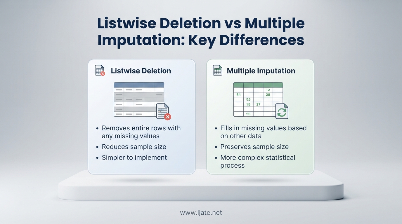
Missing data is one of the most common headaches in statistical analysis. Whether you are running a regression on survey responses, analyzing clinical trial outcomes, or building a machine learning model, incomplete rows creep into nearly every real-world dataset. The two most widely debated methods for handling this problem are listwise deletion and multiple imputation. Understanding the difference between listwise deletion and multiple imputation can make or break the validity of your results.

Listwise deletion (also called complete case analysis) simply drops every observation that has a missing value on any variable in your model. Multiple imputation, on the other hand, fills in missing values multiple times using statistical models, runs your analysis on each completed dataset, and then pools the results. One throws data away. The other tries to reconstruct it.

The choice sounds simple, but it has deep statistical implications. Pick the wrong method and you can introduce bias into your estimates, inflate your standard errors, or lose statistical power for no good reason. Researchers, data scientists, and graduate students frequently struggle with this decision because the guidance out there is often either too academic to be practical or too simplified to be accurate.

Our team has spent years working with messy datasets across social science research, health analytics, and business data projects. We have seen firsthand how the wrong missing data strategy can derail a study. This guide breaks down both methods in plain language, explains when each one wins, and gives you a practical decision framework you can actually use.

We will cover the three missingness mechanisms (MCAR, MAR, and MNAR) that determine which method is appropriate. We will walk through step-by-step workflows, compare bias and efficiency tradeoffs, provide code examples in R and Python, and answer the most common questions researchers ask when facing this decision.

Quick Reference: The Difference Between Listwise Deletion and Multiple Imputation

The core difference between listwise deletion and multiple imputation comes down to what each method does with incomplete observations. Listwise deletion removes them entirely. Multiple imputation fills them in with plausible values and accounts for the uncertainty of those guesses.

Here is a quick comparison table to orient you before we go deeper.

Feature	Listwise Deletion	Multiple Imputation
What it does	Drops rows with any missing values	Fills in missing values multiple times
Sample size	Shrinks (sometimes dramatically)	Preserved at original level
Statistical power	Reduced when missingness is high	Retained
Bias under MCAR	Unbiased	Unbiased
Bias under MAR	Biased	Unbiased (if imputation model is correct)
Bias under MNAR	Biased	Also biased (both methods struggle)
Standard errors	Correct for the subset, but larger	Account for imputation uncertainty via Rubin’s rules
Ease of implementation	Very simple (default in most software)	More complex (requires tuning and diagnostics)
Assumptions	MCAR for unbiased results	MAR for unbiased results
Best for	Small missingness fraction with MCAR data	MAR data with moderate to high missingness

If you only have a few seconds, the takeaway is this: listwise deletion is simple but wasteful and can be biased under common missingness patterns. Multiple imputation is more complex but preserves your data and produces valid results under broader conditions.

What is Listwise Deletion?

Listwise deletion is the simplest method for handling missing data. When you use listwise deletion, your statistical software scans every row in your dataset. If a row has even one missing value on any variable included in your analysis, the entire row gets dropped. Only rows with complete data on all relevant variables survive.

This method is also called complete case analysis. The name fits because you are literally analyzing only the complete cases. Most statistical software packages, including SPSS, Stata, R, and Python libraries, default to listwise deletion or make it the easiest option. That is partly why it remains the most frequently used method in published research, according to an NIH review cited over 3,100 times.

The mechanics are straightforward. If you have a dataset with 1,000 observations and 200 of them are missing on at least one variable in your regression model, listwise deletion reduces your working sample to 800 observations. The 200 incomplete rows are gone from the analysis entirely.

Advantages of Listwise Deletion

Listwise deletion has several real advantages that explain its enduring popularity. First, it is trivially easy to use. You do not need to specify a model, choose the number of imputations, tune algorithms, or run convergence diagnostics. You just let the software drop the incomplete rows and proceed.

Second, when data are missing completely at random (MCAR), listwise deletion produces unbiased estimates. The remaining complete cases are essentially a random subsample of the full dataset. Your point estimates will be correct, though your standard errors will be larger because you have fewer observations.

Third, as Paul Allison at Statistical Horizons has argued convincingly, listwise deletion can actually be less biased than multiple imputation in specific scenarios. When missingness occurs on predictor variables in a regression model and the missingness depends on the outcome variable, listwise deletion remains unbiased while multiple imputation can introduce bias. This is a point that many researchers miss.

Fourth, listwise deletion produces valid standard errors for the sample it analyzes. There is no extra layer of modeling uncertainty to account for. The standard errors you get from your regression output are honest estimates for the complete cases subset.

Disadvantages of Listwise Deletion

The problems start when data are not MCAR. Under missing at random (MAR) conditions, where the probability of missingness depends on observed variables but not on the missing value itself, listwise deletion produces biased estimates. The complete cases are no longer representative of the full population.

The bias can be substantial. Imagine a survey where older respondents are less likely to report their income. If you drop everyone with missing income, your sample skews younger, and your income estimates are systematically too low. The direction and magnitude of the bias depend on how strong the relationship is between the observed variables and missingness.

Even under MCAR, listwise deletion wastes data. If each variable in your model has a small independent missingness rate, the combined effect can be devastating. A dataset with 10 variables, each missing on 5 percent of cases, could lose 40 percent or more of its observations under listwise deletion. That translates directly into reduced statistical power and wider confidence intervals.

As Stef van Buuren notes in his comprehensive reference on missing data, listwise deletion produces standard errors that are correct for the complete case subset but generally too large for the entire dataset. You lose precision without gaining accuracy.

What is Multiple Imputation?

Multiple imputation takes a fundamentally different approach. Instead of throwing away incomplete rows, it fills in the missing values with plausible estimates. And instead of doing this once, it does it multiple times to account for the uncertainty inherent in guessing missing values.

The method was developed by Donald Rubin in the 1970s and 1980s. The core idea is elegant. Missing values are replaced with random draws from a predictive distribution based on the observed data. This process is repeated to create several complete datasets, each with slightly different imputed values. You run your analysis on each dataset separately, then combine the results using a set of formulas called Rubin’s rules.

How Multiple Imputation Works Step by Step

Step 1: Choose your imputation model. This is the statistical model that predicts missing values based on observed variables. The most common approach is multiple imputation by chained equations (MICE), also known as fully conditional specification. MICE models each variable with missing values as a function of all other variables, iterating until the imputed values stabilize.

Step 2: Generate multiple complete datasets. The standard recommendation used to be 5 imputations, but more recent guidance suggests 20 to 100 imputations depending on the fraction of missing information. Each dataset contains different imputed values because the process involves random draws from the predictive distribution.

Step 3: Analyze each completed dataset separately. Run your regression, compute your means, or fit your model on each of the imputed datasets exactly as you would on a complete dataset. You get a separate set of estimates and standard errors from each one.

Step 4: Pool the results using Rubin’s rules. The combined estimate is the average of the individual estimates across all imputed datasets. The combined standard error has two components: the within-imputation variance (the average of the individual standard errors squared) and the between-imputation variance (how much the estimates vary across datasets). This dual-component standard error honestly reflects both sampling uncertainty and imputation uncertainty.

Step 5: Check diagnostics. Examine convergence traces from MICE, look at the distribution of imputed values versus observed values, and verify that the fraction of missing information is not unreasonably high. If the imputed values look wildly different from the observed values, your imputation model may be misspecified.

Step 6: Report your methods transparently. State how many imputations you used, what imputation algorithm you chose, which variables were included in the imputation model, and what diagnostics you checked. This is increasingly expected by journal reviewers and replicability standards.

What Are Rubin’s Rules?

Rubin’s rules are the mathematical formulas that combine results across imputed datasets. The pooled point estimate is simply the average of the estimates from each dataset. The pooled variance combines within-imputation and between-imputation components.

The within-imputation variance is the average of the squared standard errors from each dataset. The between-imputation variance measures how much the point estimates bounce around across imputations. The total variance is the within-imputation variance plus a factor that inflates it based on the between-imputation variance.

This matters because it means multiple imputation gives you honest standard errors that reflect the fact that you did not actually observe those values. If your imputed values are highly uncertain, the between-imputation variance will be large, and your standard errors will be wider. This is the opposite of single imputation, which pretends that imputed values are real observations and produces artificially small standard errors.

The Fraction of Missing Information

The fraction of missing information (FMI) is a key diagnostic that comes out of Rubin’s rules. It measures how much information about a parameter is lost due to missing data. An FMI of 0 means no information was lost. An FMI of 1 means all information is missing.

The FMI is related to but not identical to the percentage of missing cases. If the observed data strongly predict the missing values, the FMI can be low even when the missingness rate is high. Conversely, if the missing values are poorly predicted, the FMI can be high even with a modest missingness rate.

Most researchers recommend using the FMI to decide how many imputations to run. A common rule of thumb is that the number of imputations should be at least as large as the largest FMI across parameters of interest. So if your maximum FMI is 0.30, you should run at least 30 imputations.

The Three Missingness Mechanisms: MCAR, MAR, and MNAR

You cannot choose between listwise deletion and multiple imputation without understanding the three missingness mechanisms. These mechanisms describe why data are missing, and they determine which methods will produce valid results.

Missing Completely at Random (MCAR)

Data are missing completely at random when the probability of a value being missing is unrelated to anything. It does not depend on the missing value itself, on any observed variable, or on any unobserved variable. A data entry error that randomly drops values is MCAR. A coin flip that determines whether a survey question appears is MCAR.

MCAR is the most restrictive assumption and the rarest in practice. When data truly are MCAR, both listwise deletion and multiple imputation produce unbiased estimates. Listwise deletion loses power, but the results are not biased. Multiple imputation retains power and also produces unbiased results.

You can test for MCAR using Little’s MCAR test, which compares the means of observed variables across groups defined by missing data patterns. If the test is not significant, you fail to reject MCAR. However, failing to reject MCAR does not prove MCAR is true. It just means you do not have strong evidence against it.

Missing at Random (MAR)

Data are missing at random when the probability of missingness depends on observed variables but not on the unobserved missing value itself. For example, if men are less likely to report their depression score than women, but within each gender the probability of missingness does not depend on the actual depression level, the data are MAR.

MAR is much more realistic than MCAR. Most researchers agree that MAR is the most defensible assumption in many real-world settings. Under MAR, listwise deletion produces biased estimates because dropping incomplete cases changes the composition of your sample in systematic ways.

Multiple imputation, however, can produce unbiased estimates under MAR if the imputation model includes the variables that predict missingness. This is why multiple imputation is generally recommended over listwise deletion when you suspect MAR.

The key insight is that MAR is an assumption, not something you can prove. You can make it more plausible by including as many relevant predictors as possible in your imputation model. The more variables you include, the more likely it is that the remaining missingness mechanism is conditionally random.

Missing Not at Random (MNAR)

Data are missing not at random when the probability of missingness depends on the unobserved value itself. For example, if people with very high incomes are less likely to report their income, and this tendency is not fully explained by observed variables, the data are MNAR.

MNAR is the hardest mechanism to handle. Neither listwise deletion nor standard multiple imputation produces unbiased estimates under MNAR. Both methods require assumptions that are violated when missingness depends on the missing value.

For MNAR data, you need specialized models that explicitly model the missingness mechanism. These include selection models, pattern mixture models, and shared parameter models. These approaches are complex, require strong assumptions, and are sensitive to model specification.

The honest truth is that you can never definitively determine whether your data are MAR or MNAR from the data alone. Both mechanisms produce identical observed data patterns. You need substantive knowledge about your domain to argue for one over the other.

Missingness Mechanisms Comparison Table

Mechanism	Definition	Listwise Deletion	Multiple Imputation	Realism
MCAR	Missingness unrelated to anything	Unbiased (loses power)	Unbiased (retains power)	Rare
MAR	Missingness explained by observed data	Biased	Unbiased (if model is correct)	Plausible
MNAR	Missingness depends on missing value	Biased	Biased (standard MI fails)	Common but hard to detect

Listwise Deletion vs Multiple Imputation: Side-by-Side Comparison

Now that we understand the building blocks, let us compare listwise deletion and multiple imputation head to head across the dimensions that matter most for your research.

Bias

Bias is the most important criterion. A biased estimate is wrong on average, no matter how precise it appears. Listwise deletion is unbiased only under MCAR. Multiple imputation is unbiased under both MCAR and MAR (assuming the imputation model is correctly specified). Under MNAR, both methods are biased.

The bias from listwise deletion under MAR can be severe. If 20 percent of your data are missing on a variable and that missingness is related to observed characteristics, dropping those cases can shift your estimates substantially. The Cambridge study by Pepinsky (2018) demonstrated this with simulation evidence, showing that listwise deletion produced biased regression coefficients under MAR conditions while multiple imputation recovered the true values.

However, Paul Allison makes an important counterpoint. When missingness is on a predictor variable in a regression and the missingness mechanism depends on the outcome variable, listwise deletion is actually unbiased. Multiple imputation, in this specific scenario, can introduce bias because it models the predictor as a function of the outcome, which changes the conditional distribution. This is a nuanced but important exception.

Statistical Power and Efficiency

Statistical power is your ability to detect true effects. Listwise deletion reduces power by reducing sample size. Multiple imputation retains power by keeping all observations in the analysis.

The efficiency loss from listwise deletion depends on how much data you lose. With 5 percent missingness spread across variables, you might lose 15 to 25 percent of your cases. With 20 percent missingness, you could lose over half your sample. Each dropped case represents lost information.

Multiple imputation is more efficient than listwise deletion even under MCAR. The imputed values contribute information, reducing the variance of your estimates. Under MAR, the efficiency advantage is even larger because listwise deletion is both biased and inefficient.

Standard errors tell a similar story. Listwise deletion standard errors are valid for the reduced sample but are larger than they need to be. Multiple imputation standard errors, computed via Rubin’s rules, account for imputation uncertainty but are still generally smaller than listwise deletion standard errors because they use more data.

Assumptions

Both methods require assumptions, but they differ in what they assume. Listwise deletion assumes MCAR for unbiased results. This is a strong assumption that is rarely fully met in practice.

Multiple imputation assumes MAR for unbiased results. MAR is weaker and more plausible than MCAR, but it is still an assumption you must justify. Multiple imputation also assumes that your imputation model is correctly specified. If you leave out important predictors of missingness, your imputed values will be off.

Both methods assume that the missingness mechanism is ignorable, meaning you do not need to model it explicitly. Under MNAR, this assumption fails, and neither method is sufficient without extensions.

Ease of Implementation

Listwise deletion wins hands down on simplicity. It is the default in most statistical software. You do nothing special. You just run your analysis and the software handles the missing data by dropping incomplete rows.

Multiple imputation requires more effort. You need to choose an imputation method (MICE is most common), decide how many imputations to create, select variables for the imputation model, run convergence diagnostics, and pool results correctly. In R, the mice package makes this manageable. In SPSS, multiple imputation is built in but requires clicking through dialog boxes. In Python, libraries like scikit-learn and statsmodels offer imputation tools but with less built-in support for Rubin’s rules.

Forum discussions on Reddit and StackExchange reveal that many researchers find multiple imputation intimidating. Graduate students especially report struggling with MICE convergence issues and uncertainty about whether their imputation model is appropriate. This is a real practical barrier that keeps people using listwise deletion even when multiple imputation would be better.

Reproducibility and Transparency

Multiple imputation introduces a reproducibility challenge that listwise deletion does not. Because imputation involves random draws, different runs can produce slightly different results unless you set a random seed. You should always set a seed and report it.

On the other hand, multiple imputation is more transparent about its assumptions. You explicitly state your imputation model, the number of imputations, and diagnostics. Listwise deletion hides behind a default that many researchers never question or even mention.

Comprehensive Comparison Table

Criterion	Listwise Deletion	Multiple Imputation
Unbiased under MCAR	Yes	Yes
Unbiased under MAR	No	Yes (with correct imputation model)
Unbiased under MNAR	No	No
Retains sample size	No	Yes
Statistical power	Reduced	Retained
Standard errors	Valid but larger	Valid and smaller (Rubin’s rules)
Implementation difficulty	Very easy	Moderate to advanced
Software support	Universal default	Built into R, SPSS, Stata; Python growing
Requires random seed	No	Yes
Diagnostic requirements	Minimal	Convergence checks, FMI, distribution plots
Publication acceptance	Increasingly questioned	Increasingly expected

Bias and Efficiency: When Each Method Succeeds or Fails

Let us go deeper into the statistical properties that determine when each method is appropriate. This is where the research literature gets technical, but the core ideas are accessible if we break them down.

When Listwise Deletion Is Unbiased

Listwise deletion produces unbiased estimates when the complete cases are a random sample of the full dataset. This happens under MCAR, where missingness is independent of everything. It also happens in a less obvious scenario that Allison highlighted: when missingness occurs only on predictor variables in a regression and depends only on the outcome variable.

The second scenario is surprisingly common. Imagine predicting college GPA from high school GPA and test scores, where some students do not report their test scores. If the probability of not reporting depends on GPA (the outcome) but not on the test score itself, listwise deletion gives you unbiased regression coefficients for the other predictors.

This does not mean listwise deletion is always fine for missing predictors. It is fine specifically when the missingness mechanism satisfies certain conditions. The point is that the blanket statement “listwise deletion is always bad” is an oversimplification.

When Listwise Deletion Produces Severe Bias

Under MAR, listwise deletion can produce substantial bias. The magnitude depends on how strongly the observed variables predict missingness and how different the complete cases are from the dropped cases.

Pepinsky’s 2018 simulation study showed that under MAR conditions, listwise deletion produced regression coefficients that deviated significantly from the true values. The bias was large enough to change substantive conclusions in some scenarios. Multiple imputation, using the same data and correctly specified models, recovered the true coefficients.

The practical implication is this: if you suspect that the probability of missingness is related to any observed variable in your dataset, listwise deletion is risky. The bias may not be obvious from looking at your results. You need to think carefully about the missingness mechanism.

When Multiple Imputation Can Be Worse Than Listwise Deletion

This may surprise you, but multiple imputation is not always better. There are documented scenarios where MI produces worse results than listwise deletion.

First, under MNAR conditions where standard imputation models are used, multiple imputation can amplify bias rather than reduce it. The imputed values are based on incorrect assumptions about the missingness mechanism, and these incorrect values can pull estimates further from the truth. Pepinsky’s simulations showed that under certain MNAR scenarios, listwise deletion had lower mean squared error than multiple imputation.

Second, when the proportion of missing data is very small (under 5 percent), the gain from multiple imputation is negligible while the cost in complexity is real. The NIH review notes that multiple imputation may be unnecessary when missingness is this small, especially under MCAR.

Third, a poorly specified imputation model can be worse than no imputation at all. If you leave out variables that predict missingness, include inappropriate variables, or fail to achieve convergence, your imputed values can introduce bias that listwise deletion would not have.

Coverage Rates and Confidence Interval Performance

Coverage rate is the percentage of times your confidence interval contains the true parameter value across repeated samples. A nominal 95 percent confidence interval should contain the true value 95 percent of the time.

Under MCAR, both listwise deletion and multiple imputation achieve approximately nominal coverage. Under MAR, listwise deletion coverage drops because the point estimates are biased. Even though the confidence intervals are centered on the wrong value, the intervals themselves may be narrow enough to exclude the true value.

Multiple imputation maintains nominal coverage under MAR if the imputation model is correct. The between-imputation variance widens the intervals to account for imputation uncertainty, which helps maintain proper coverage. This is one of the key advantages of MI over single imputation methods.

Mean Squared Error Comparison

Mean squared error (MSE) combines bias and variance into a single metric. Lower MSE means better estimates overall. Under MCAR, listwise deletion has higher MSE than multiple imputation because it has larger variance from the reduced sample size but similar bias.

Under MAR, listwise deletion has much higher MSE because it has both bias and large variance. Multiple imputation has lower MSE if the imputation model is well specified. Under MNAR, the comparison is unclear and depends on the specific scenario and model choices.

The MSE framework is helpful because it reminds us that bias is not the only thing that matters. Even if listwise deletion were unbiased (under MCAR), it would still have larger MSE due to variance inflation from the smaller sample.

When to Use Listwise Deletion vs Multiple Imputation

Let us turn the statistical theory into a practical decision framework. Here is how to choose between listwise deletion and multiple imputation in real research situations.

Use Listwise Deletion When

Use listwise deletion when your missing data fraction is small. If fewer than 5 percent of cases have missing values on any variable in your model, the impact on your results will be minimal regardless of which method you use. The simplicity of listwise deletion wins in this scenario.

Use listwise deletion when you have strong evidence that data are MCAR. If Little’s MCAR test is not significant and you have substantive reasons to believe missingness is truly random, listwise deletion will give you unbiased estimates. Just be aware that failing to reject MCAR is not the same as proving it.

Use listwise deletion when missingness is on predictor variables only and you have a large sample. Allison’s work shows that in this specific scenario, listwise deletion can be unbiased even under certain non-MCAR patterns. If losing some cases does not threaten your statistical power, the simplicity is worth it.

Use listwise deletion as a sensitivity analysis alongside multiple imputation. Run both methods and compare results. If they agree, your conclusions are robust. If they disagree, investigate why and report both sets of results.

Use Multiple Imputation When

Use multiple imputation when you suspect data are MAR. This covers most real-world datasets. If the probability of missingness on any variable plausibly depends on other observed variables, multiple imputation will give you less biased estimates than listwise deletion.

Use multiple imputation when the missing data fraction is moderate to high. If 10 to 40 percent of cases have missing values, listwise deletion will strip too much data and undermine your statistical power. Multiple imputation preserves your sample size and produces more efficient estimates.

Use multiple imputation when missingness occurs on the outcome variable. Dropping cases with missing outcomes under MAR introduces bias. Multiple imputation can recover the missing outcomes using observed predictor variables, producing unbiased estimates.

Use multiple imputation when journal reviewers or funding agencies expect it. Increasingly, methodological standards in health research, social sciences, and psychology expect researchers to justify their missing data handling. Multiple imputation signals methodological rigor.

Avoid Both Methods When

If the fraction of missing data exceeds 40 to 50 percent, neither method is reliable. Multiple imputation becomes unstable with high missingness rates, and listwise deletion may leave you with too few cases to analyze. In these situations, consider whether your dataset can support the analysis at all.

If you suspect MNAR, both methods are biased. You need specialized approaches like selection models or pattern mixture models. Consult a statistician, as these methods require expertise to implement correctly.

If your analysis requires categorical variables with many levels or interactions, multiple imputation becomes more complex. MICE can handle these cases but requires careful specification. Take the time to understand how your software handles these situations.

Decision Framework in Plain Language

Step 1: Assess how much data are missing. If under 5 percent, listwise deletion is probably fine. If over 40 percent, rethink your analysis.

Step 2: Think about why data are missing. If missingness seems random, MCAR is plausible and listwise deletion works. If missingness relates to observed variables, MAR is more likely and multiple imputation is better.

Step 3: Check where missingness occurs. If only predictors are missing and you have a large sample, listwise deletion may be acceptable. If outcomes or key variables are missing, lean toward multiple imputation.

Step 4: Consider your audience. If reviewers or collaborators expect rigorous missing data handling, multiple imputation demonstrates thoroughness. If you are doing exploratory analysis, listwise deletion may be sufficient for now.

Step 5: Run both methods as a sensitivity check. Compare results. Report both if they differ. This is the most defensible approach and will satisfy most reviewers.

Practical Implementation in R, Python, SPSS, and Stata

Theory is helpful, but at some point you need to actually run the analysis. Here is practical guidance for implementing both methods in common statistical software.

Listwise Deletion

In R, listwise deletion happens automatically with most modeling functions. The lm() function drops rows with missing values by default. You can also explicitly use na.omit() on your dataframe. In Python, pandas and statsmodels also default to dropping missing values.

In SPSS, listwise deletion is the default for most procedures. You do not need to do anything special. In Stata, the regress command automatically drops incomplete cases. This is part of why listwise deletion is so common. It requires zero effort.

Multiple Imputation in R

The mice package in R is the gold standard for multiple imputation. The basic workflow is to call mice() on your data, which creates multiple imputed datasets stored in a special object. You then run with() to apply your analysis function to each dataset, and pool() to combine the results using Rubin’s rules.

A typical R session would look like: install and load the mice package, run the mice() function on your dataset specifying the number of imputations (commonly 20 to 50), use the with() function to fit your model on each imputed dataset, and then call pool() to get combined estimates with appropriate standard errors. The mice package also provides diagnostic plots to check convergence and compare imputed versus observed distributions.

The Amelia package is another option, particularly good for time-series cross-sectional data. It uses a different algorithm (bootstrapped EM) but follows the same multiple imputation principle.

Multiple Imputation in Python

Python has been catching up on multiple imputation support. The scikit-learn library offers SimpleImputer and IterativeImputer (which is similar to MICE). However, scikit-learn does not natively support Rubin’s rules for pooling results.

The statsmodels library has some experimental imputation functionality. For full multiple imputation with Rubin’s rules in Python, you may need to implement the pooling manually or use a wrapper. The workflow is less streamlined than in R, which is why many Python users still turn to R for serious missing data work.

Multiple Imputation in SPSS and Stata

SPSS has a built-in multiple imputation module accessible through the Analyze menu. You specify the variables, choose the imputation method (fully conditional specification is the default, equivalent to MICE), set the number of imputations, and SPSS creates a special dataset with an imputation identifier variable. You then run your analysis on this dataset, and SPSS automatically pools the results.

Stata has the mi suite of commands for multiple imputation. You declare your data as mi data, impute using mi impute (which supports chained equations), run your analysis with mi estimate, and Stata handles the pooling. Stata’s implementation is well-documented and user-friendly.

Software Comparison Tips

If you have a choice, R with the mice package offers the most flexibility and the best diagnostics. Stata’s mi commands are also excellent and well-integrated. SPSS is fine for standard analyses but less flexible for complex models. Python is improving but still lags in native Rubin’s rules support.

Regardless of which software you use, always set a random seed before running multiple imputation. This ensures reproducibility. Report the seed in your methods section so others can replicate your results exactly.

Pairwise Deletion: A Third Alternative Worth Knowing

Listwise deletion and multiple imputation get the most attention, but pairwise deletion is a third method that appears in related searches and is worth understanding.

Pairwise deletion (also called available case analysis) uses all available data for each pairwise calculation. When computing a correlation matrix, for example, pairwise deletion uses every case that has complete data on the two variables involved in each correlation. This means different correlations in the matrix may be based on different subsets of the data.

The advantage of pairwise deletion is that it retains more data than listwise deletion. The disadvantage is that it can produce inconsistent results. Correlation matrices computed with pairwise deletion may not be positive definite, which means you cannot fit a regression or factor analysis model to them. Standard errors from pairwise deletion are also difficult to compute correctly because the effective sample size varies across pairs.

Most statisticians recommend avoiding pairwise deletion for primary analyses. It can be useful for exploratory data visualization or as a comparison point, but it should not be your main missing data strategy. Multiple imputation handles the same situations more rigorously by imputing the missing values and maintaining a consistent sample size across all analyses.

Common Misconceptions About Listwise Deletion and Multiple Imputation

Several myths about these methods circulate in graduate programs, online forums, and even published papers. Let us address the most common ones.

Misconception 1: Listwise Deletion Is Always Wrong

This is the most pervasive myth. The “listwise deletion is evil” narrative, often attributed to King et al. (2001), has been repeated so often that many researchers treat it as gospel. But as Allison and others have shown, listwise deletion is unbiased under MCAR and can outperform multiple imputation in specific scenarios. The truth is more nuanced than the slogan.

Listwise deletion is a legitimate method when its assumptions are met. The problem is that researchers use it by default without checking those assumptions. The solution is not to ban listwise deletion but to use it thoughtfully.

Misconception 2: Multiple Imputation Always Produces Better Results

Multiple imputation is not magic. It depends on the correctness of the imputation model, the plausibility of the MAR assumption, and the quality of the observed data. A poorly executed multiple imputation can be worse than listwise deletion.

Multiple imputation also adds a layer of complexity that can go wrong. Convergence failures, inappropriate variable transformations, and missing important interactions in the imputation model can all degrade results. The method is only as good as its implementation.

Misconception 3: You Need Hundreds of Imputations

Older guidance suggested 5 imputations were sufficient. Newer guidance suggests more, especially when the fraction of missing information is high. But you do not need hundreds. A practical rule is to set the number of imputations equal to the percentage of incomplete cases, up to about 100. For most analyses, 20 to 50 imputations is plenty.

Misconception 4: You Can Prove MCAR

Little’s MCAR test can fail to reject MCAR, but this does not prove MCAR is true. It just means your test was not powerful enough to detect deviations. You should treat MCAR as a working assumption, not a proven fact. If you have substantive reasons to believe missingness depends on observed variables, assume MAR and use multiple imputation.

Misconception 5: Multiple Imputation Fixes All Missing Data Problems

Multiple imputation handles MCAR and MAR but not MNAR. If your data are missing not at random, standard multiple imputation will still give you biased results. You need specialized models for MNAR data, and even those require assumptions you cannot verify from the data.

The honest answer is that no missing data method is a complete fix. The best strategy is to minimize missingness during data collection, understand why missingness occurred, and choose your method based on the most plausible mechanism.

How to Report Your Missing Data Method

Whatever method you choose, you need to report it clearly. Journal reviewers, collaborators, and future replicators need to understand what you did. Here is what to include.

Report the amount of missing data. State the percentage of cases with missing values on each variable and overall. Report the pattern of missingness (which variables tend to be missing together).

State which method you used and why. If you used listwise deletion, explain why you believe the assumption (MCAR or the predictor-only missingness condition) is reasonable. If you used multiple imputation, specify the imputation algorithm (MICE, Amelia, etc.), the number of imputations, the variables included in the imputation model, and any transformations.

Report diagnostics. For multiple imputation, mention convergence checks, the fraction of missing information, and comparisons of imputed versus observed distributions. If you ran sensitivity analyses with both methods, report both sets of results.

Be transparent about limitations. Acknowledge the missingness mechanism you assumed and the possibility that it is wrong. This is good scientific practice and will strengthen your paper, not weaken it.

FAQs

Conclusion

The difference between listwise deletion and multiple imputation comes down to a tradeoff between simplicity and validity. Listwise deletion is easy to implement and works well when data are MCAR or when missingness is limited to predictors in regression. Multiple imputation is more complex but produces unbiased and efficient estimates under the broader and more realistic MAR condition.

Neither method is universally superior. The right choice depends on your missingness mechanism, the amount of missing data, where missingness occurs, your statistical power needs, and the expectations of your audience. The best researchers do not reflexively choose one method. They think carefully about the data, test their assumptions, and often run sensitivity analyses with both approaches.

If you take away one thing from this guide, let it be this: your choice of missing data method directly affects the validity of your conclusions. Invest the time to understand your missingness mechanism. Run Little’s MCAR test. Compare results from both methods. Report your methods transparently. Your research will be stronger for it.