
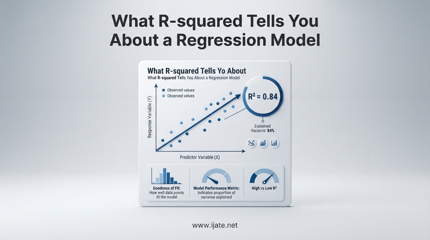
If you have ever built a regression model and stared at the output wondering what that R-squared number actually means, you are in the right place. R-squared is one of the most reported statistics in regression analysis, yet it is also one of the most misunderstood. Our team has spent years building, evaluating, and explaining regression models across fields from finance to psychology, and we have seen every common confusion firsthand. This guide breaks down exactly what R-squared tells you about a regression model, what it does not tell you, and how to use it without getting misled.
We will cover the definition, the math behind it, a step-by-step worked example with real numbers, interpretation guidelines for every range of values, field-specific benchmarks, and the limitations that competitors often gloss over. By the end, you will know how to read an R-squared value with confidence and when to question it.
Table of Contents
Quick Answer: What R-squared Tells You About a Regression Model
R-squared (R2), also called the coefficient of determination, tells you the proportion of the variance in the dependent variable that is explained by the independent variable(s) in a regression model. It ranges from 0 to 1, where 0 means the model explains none of the variation in the outcome and 1 means it explains all of it. In simple terms, an R-squared of 0.80 means that 80% of the variability in your response variable is accounted for by your predictors, and the remaining 20% is unexplained variation or noise.
What Is R-squared?
R-squared is a goodness-of-fit measure for a regression model. It quantifies how well the fitted regression line (or hyperplane, in multiple regression) captures the pattern in the observed data. The statistic was introduced by the geneticist Sewall Wright in 1921 and has since become a standard output of virtually every statistical software package, from Excel and SPSS to R, Python’s scikit-learn, and Stata.
Think of it this way: your dependent variable has some total variation, meaning the observed values spread around their mean. A regression model tries to explain that spread using one or more predictor variables. R-squared reports what fraction of that total spread the model successfully accounts for. The closer R-squared is to 1, the tighter the data points cluster around the fitted regression line.
A common point of confusion is why the statistic is “squared.” The name comes from the fact that, in simple linear regression with one predictor, R-squared literally equals the square of the Pearson correlation coefficient (r) between the predictor and the response. If the correlation r is 0.9, then R-squared is 0.81. Squaring the correlation converts a linear association strength into a proportion of variance explained, which is often a more meaningful scale for interpretation.
It is worth noting that R-squared alone never tells you whether your model is correct, whether your predictors are statistically significant, or whether you have chosen the right functional form. It only tells you how much variance the model explains, given its current specification. That distinction matters enormously in practice, and we will return to it throughout this guide.
How R-squared Is Calculated
The standard formula for R-squared is R2 = 1 minus (SSres / SStot). Here, SSres is the residual sum of squares (the sum of squared differences between the observed values and the values predicted by the model), and SStot is the total sum of squares (the sum of squared differences between the observed values and their mean). In other words, R-squared compares the variation your model leaves unexplained (the residuals) against the total variation that existed in the data to begin with.
If your model predicts perfectly, every residual is zero, SSres is zero, and R-squared equals 1. If your model is no better than just guessing the mean of the dependent variable for every observation, then SSres equals SStot and R-squared equals 0. This is the core intuition: R-squared measures how much better your model is than a flat baseline that ignores all predictors.
Step-by-Step Worked Example
Let us walk through a concrete calculation with a tiny dataset. Suppose we have five observations of a predictor X and a response Y.
Our data: X = [1, 2, 3, 4, 5] and Y = [2, 4, 5, 4, 5]. First, compute the mean of Y, which is (2 + 4 + 5 + 4 + 5) / 5 = 4. Next, fit a simple linear regression using ordinary least squares. The fitted line turns out to be Y-hat = 2.6 + 0.6X, giving predicted values of [3.2, 3.8, 4.4, 5.0, 5.6].
Now compute the residuals (observed minus predicted): [2 – 3.2, 4 – 3.8, 5 – 4.4, 4 – 5.0, 5 – 5.6] = [-1.2, 0.2, 0.6, -1.0, -0.6]. Square each residual: [1.44, 0.04, 0.36, 1.00, 0.36]. Sum them to get SSres = 3.20.
Next compute the total sum of squares. Subtract the mean (4) from each Y value: [-2, 0, 1, 0, 1]. Square those: [4, 0, 1, 0, 1]. Sum them to get SStot = 6.
Finally, R-squared = 1 – (SSres / SStot) = 1 – (3.20 / 6) = 1 – 0.5333 = 0.4667. So this simple model explains about 46.7% of the variance in Y. That is a small example, but the same logic scales to datasets of any size and to multiple regression with many predictors.
Interpreting R-squared Values
R-squared lives on a scale from 0 to 1, and different ranges carry different practical meanings. There is no universal cutoff that separates a “bad” model from a “good” one, because the right answer depends heavily on your field, your data, and your goals. Still, having a sense of what each range typically signals helps you read the number quickly.
R-squared Near 1.0 (0.90 and Above)
An R-squared above 0.90 means the model explains over 90% of the variance in the response variable. In the physical sciences and engineering, where measurements are precise and relationships follow well-understood laws, values this high are expected and normal. In the social sciences or behavioral research, an R-squared this high is a red flag worth investigating. It can indicate overfitting, data leakage, a tautological model where a predictor is essentially a restatement of the outcome, or measurement that is too close to deterministic to be informative.
R-squared Between 0.7 and 0.9
This range is generally considered strong across most applied fields. A model explaining 70% to 90% of the variance is capturing the dominant patterns in the data while leaving a modest amount of unexplained noise. In business forecasting, sales modeling, and many engineering applications, this is the sweet spot practitioners aim for. Always pair it with a residual plot inspection to confirm the model is not hiding systematic bias.
R-squared Between 0.5 and 0.7
A model in this range explains about half to two-thirds of the variance in the outcome. This is perfectly respectable in many fields, especially those involving human behavior, survey data, or noisy real-world processes. In marketing analytics, operations research, and epidemiology, R-squared values in this band are common and useful. The model is capturing meaningful structure even though substantial variation remains unexplained.
R-squared Between 0.2 and 0.5
Here the model explains 20% to 50% of the variance. In psychology, education research, and many areas of medicine, this range is entirely normal and the model may still be highly valuable. What matters is whether the predictors are statistically significant and whether the effect sizes are practically meaningful. A low R-squared with strong, interpretable predictors often tells you that the phenomenon you are studying is genuinely complex and influenced by many factors outside your dataset.
R-squared Below 0.2
An R-squared under 0.20 means the model explains less than a fifth of the variance. This does not automatically make the model useless. In fields like stock market prediction, genomics, or early-stage social science research, low R-squared values are routine because the systems being modeled are inherently noisy. The relevant question is whether your model still beats a naive baseline and whether the predictors you identified carry real, replicable signal.
What an R-squared of 0.5 Means Specifically
An R-squared of exactly 0.5 means your model explains half of the variance in the dependent variable. The other half comes from factors your model does not capture, including unmeasured predictors, measurement error, and pure randomness. Whether 0.5 is good or bad depends entirely on context: it would be a weak result in a physics experiment measuring a deterministic relationship, but a strong result in a psychology study predicting human behavior.
What an R-squared of 1.0 Means Specifically
An R-squared of exactly 1 means the model fits the data perfectly, with every observation falling exactly on the fitted regression line. In real-world data, a perfect R-squared almost always signals a problem rather than a triumph. It typically means the model is overfit, a predictor variable is a deterministic function of the response, or there is data leakage. Treat a perfect R-squared as a warning to investigate, not a celebration.
Can R-squared Be Negative?
Yes. R-squared can go negative when a model fits the data worse than a horizontal line drawn at the mean of the dependent variable. This happens most often with non-linear models evaluated on the same formula, or when a model trained on one dataset is evaluated on a different dataset where it performs poorly. A negative R-squared tells you the model is actively worse than predicting the mean, which is a clear signal to reconsider your approach.
What Is a Good R-squared Value?
The honest answer is that “good” depends on your field, your data, and your purpose. There is no universal threshold. A value that would be considered excellent in psychology might be considered poor in physics, and vice versa. The most useful question is not “is my R-squared high enough?” but “is my R-squared reasonable for the kind of problem I am working on?”
Forum discussions on Reddit’s r/statistics and r/AskStatistics consistently surface this exact confusion. Analysts new to regression often ask whether an R-squared of 0.30 or 0.50 is acceptable, and experienced practitioners always respond the same way: it depends on the field. To make this concrete, here are typical R-squared benchmarks by discipline.
Field-Specific R-squared Benchmarks
In physics and the hard physical sciences, R-squared values above 0.90 or even 0.95 are often expected because the systems follow deterministic laws and measurement error is small. In engineering and manufacturing process control, R-squared values between 0.70 and 0.95 are common and desirable. In finance and econometrics, where markets are noisy, R-squared between 0.30 and 0.60 is often the realistic ceiling for predictive models. In marketing and business analytics, values between 0.40 and 0.70 are typical for well-specified models. In psychology, education, and the social sciences, R-squared between 0.20 and 0.50 is normal and publishable. In early-stage biomedical research and genomics, R-squared below 0.20 is routine because biological systems are extraordinarily complex.
These benchmarks are guidelines, not rules. A model with a lower R-squared than the typical range for its field can still be valuable if the predictors are theoretically important and the effect sizes are practically meaningful. Conversely, a model with a higher R-squared than expected deserves scrutiny for possible overfitting or specification problems.
When Low R-squared Is Acceptable
Low R-squared is acceptable and even expected in several scenarios. First, when you are studying inherently noisy phenomena like human behavior, financial markets, or biological systems, no model will capture most of the variance. Second, when your goal is to identify the effect of a specific predictor rather than to maximize prediction accuracy, even a low R-squared can support a meaningful conclusion. Third, when you are working in an early exploratory phase and building theory rather than predicting outcomes, modest explanatory power is fine. Fourth, when the predictors you are testing are statistically significant and replicable across studies, the model contributes real knowledge even if it leaves most variance unexplained.
When High R-squared Is Misleading
High R-squared can be misleading just as easily as low R-squared. A model with an R-squared of 0.98 can still be a bad fit if the residuals show a systematic pattern, such as a curved shape that indicates the model is missing a nonlinear term. This is called specification bias. High R-squared can also result from overfitting, where the model has memorized the training data rather than learning a generalizable pattern. Time-series data often produce inflated R-squared values because of shared trends rather than genuine causal relationships. And in some cases, a high R-squared simply reflects a tautological model where one predictor is essentially a restatement of the outcome variable.
This is why experienced analysts always inspect residual plots alongside the R-squared value. A residual plot with no pattern (random scatter around zero) supports the model. A residual plot with curvature, funneling, or trend tells you the model is missing something, regardless of how high the R-squared looks.
Limitations and Caveats of R-squared
R-squared is a useful statistic, but relying on it alone leads to bad models. Understanding its limitations is essential for any practitioner.
1. R-squared Always Increases When You Add Predictors
Every time you add a new predictor to a regression model, R-squared goes up or stays the same. It never decreases, even if the added variable is pure noise. This makes R-squared a poor tool for model comparison when the models have different numbers of predictors. A model with ten predictors will almost always have a higher R-squared than a model with two, regardless of whether those extra predictors carry any real signal. This is exactly why adjusted R-squared exists, and we cover it in the next section.
2. R-squared Does Not Detect Specification Bias
R-squared cannot tell you whether you have chosen the correct functional form for your model. You can have a high R-squared while missing an important quadratic term, an interaction effect, or an entirely omitted variable. The residuals, not the R-squared, reveal these problems. A model can look great on R-squared while systematically over-predicting in one range and under-predicting in another.
3. R-squared Does Not Indicate Statistical Significance
A high R-squared does not mean your predictors are statistically significant, and a low R-squared does not mean they are not. You must check p-values, confidence intervals, and F-tests separately. A model with a modest R-squared of 0.30 can have highly significant, theoretically important predictors, while a model with a high R-squared of 0.90 can include variables that are not individually significant.
4. R-squared Is Sensitive to Outliers
A single extreme observation can dramatically inflate or deflate R-squared. Always examine your data for outliers and influential points before trusting the statistic. Leverage points (extreme predictor values) and high-residual observations can both distort R-squared in ways that mislead.
5. R-squared Does Not Generalize to New Data
R-squared computed on training data is an optimistic estimate of how well the model will perform on new data. In machine learning workflows, this is the training-versus-generalization gap. A model can have a training R-squared of 0.85 and a test R-squared of 0.40 because of overfitting. This is why cross-validation and held-out test sets matter. The concept of R-squared shrinkage captures how much the value drops when moving from training to test data, and large shrinkage signals overfitting.
6. R-squared Is Not Comparable Across Different Dependent Variables
You cannot directly compare the R-squared of a model predicting house prices against the R-squared of a model predicting mortgage default probability. The metric only makes sense within the context of a specific outcome variable measured on a specific scale. Cross-model comparisons using R-squared require the same dependent variable and the same dataset.
Adjusted R-squared Explained
Adjusted R-squared is a modified version of R-squared that penalizes the addition of predictors that do not improve the model. Unlike regular R-squared, adjusted R-squared can decrease when you add a variable that contributes less than would be expected by chance. This makes it far more useful for comparing models with different numbers of predictors and for feature selection.
The formula for adjusted R-squared is: 1 – [(1 – R2) * (n – 1) / (n – k – 1)], where n is the number of observations and k is the number of predictors. The penalty term (n – 1) / (n – k – 1) grows as you add predictors, which is what creates the downward pressure on the statistic when useless variables enter the model.
Use adjusted R-squared whenever you are comparing models with different numbers of predictors, performing stepwise selection, or deciding whether an additional variable is worth including. If adding a variable increases adjusted R-squared, it is earning its place. If adding a variable decreases adjusted R-squared, it is adding noise without explanatory value.
R-squared vs Adjusted R-squared vs Predicted R-squared
Regular R-squared measures how well the model fits the data it was trained on. It is optimistic and always increases with more predictors. Adjusted R-squared applies a penalty for model complexity, making it better for comparing models with different predictor counts. Predicted R-squared, also called press R-squared, estimates how well the model will predict new data by systematically removing observations and measuring prediction error. Predicted R-squared is the most conservative of the three and is closely related to cross-validated performance.
In practice, look at all three. A large gap between regular R-squared and predicted R-squared is a strong indicator of overfitting. A model where adjusted and predicted R-squared are close to regular R-squared is a model that generalizes well.
Pseudo-R-squared in Logistic Regression
R-squared, as classically defined, applies to ordinary least squares regression with a continuous outcome. In logistic regression, where the outcome is binary, the classic R-squared does not directly apply. Instead, statisticians use pseudo-R-squared measures such as McFadden’s R-squared, Cox and Snell’s R-squared, and Nagelkerke’s R-squared. These metrics attempt to provide an analogous “variance explained” interpretation, but they are calculated differently and generally produce lower values than classic R-squared. McFadden’s R-squared of 0.20 to 0.40 is considered an excellent fit, which is a very different scale from OLS regression. Do not compare pseudo-R-squared values directly to OLS R-squared values.
Practical Guidelines for Using R-squared
Here is a practical decision framework for evaluating whether your R-squared value is meaningful for your situation.
First, always pair R-squared with a residual plot. If the residuals show random scatter, the model specification is reasonable. If they show a pattern, fix the model before worrying about the R-squared number. Second, compare R-squared to the typical range for your field. Use the benchmarks above as a starting point, but talk to experienced practitioners in your domain. Third, check adjusted R-squared alongside regular R-squared. If the gap is large, your model may be overfit. Fourth, if you have enough data, compute a cross-validated or test-set R-squared to estimate real-world performance. Fifth, check that your predictors are statistically significant and theoretically meaningful, not just numerically present.
R-squared is a starting point for evaluating model fit, not the final word. It tells you one important thing (how much variance the model explains) and stays silent on everything else (correct specification, significance, generalization, causal validity). Treat it as one tool in a larger diagnostic toolkit.
FAQs
What does R-squared tell us about a regression model?
R-squared tells you the proportion of the variance in the dependent variable that is explained by the independent variable(s) in your regression model. It ranges from 0 to 1, where 0 means the model explains none of the variation and 1 means it explains all of it.
What is a good R2 score for a regression model?
There is no universal good R-squared value because the answer depends on your field. In physics and engineering, values above 0.90 are expected. In the social sciences and psychology, values between 0.20 and 0.50 are normal and publishable. In finance, 0.30 to 0.60 is realistic. Compare your value to the typical range for your discipline rather than chasing a universal threshold.
What does a R2 of 0.5 mean?
An R-squared of 0.5 means your model explains exactly half of the variance in the dependent variable. The remaining 50% comes from unmeasured factors, measurement error, and random noise. Whether 0.5 is good depends on context: it is weak for a deterministic physics experiment but strong for a behavioral study.
What does a R2 value of 1 mean?
An R-squared of 1 means the model fits the data perfectly, with every observation falling exactly on the fitted line. In real-world data, this almost always signals a problem such as overfitting, data leakage, or a tautological predictor rather than a genuinely perfect model.
Conclusion: What R-squared Tells You About a Regression Model
R-squared is a measure of how much variance in the dependent variable your regression model explains, and it is most useful when paired with residual diagnostics, adjusted R-squared, and field-specific context. Understanding what R-squared tells you about a regression model means knowing both its strengths and its blind spots. Use it as a starting point, not a final verdict, and always ask whether your model makes theoretical sense beyond the number on the screen.
If you take away one lesson, let it be this: a high R-squared is not automatically good, a low R-squared is not automatically bad, and no single statistic can tell you whether your model is right. The best analysts read R-squared alongside residuals, significance tests, and cross-validated performance to build models that are both accurate and honest.