
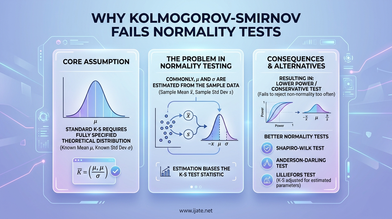
The Kolmogorov-Smirnov test is one of the most widely used statistical tools for checking normality, yet research consistently shows it is often the wrong choice. Multiple peer-reviewed studies, including a highly cited 2012 paper by Ghasemi et al. published in the Journal of Applied Statistics, conclude that the KS test should no longer be used for normality testing because of its low statistical power. If you are running a t-test, ANOVA, or linear regression and relying on the KS test to verify your normality assumption, you may be missing real violations that undermine your results. This article explains exactly why the KS test falls short, when the problem gets worse rather than better, and which normality tests you should be using instead.
Normality checks matter because most classical statistical methods assume your data or residuals follow a Gaussian distribution. When that assumption is violated, p-values become unreliable, confidence intervals lose coverage, and your conclusions may be misleading. The problem is that different normality tests tell very different stories about the same dataset, and the KS test is the least reliable of the commonly used options.
I have spent years working with researchers who run normality tests as a routine step in their analysis pipeline. What I see repeatedly is the KS test failing to flag clearly non-normal data, or flagging data as non-normal when the deviation is so small it would never affect downstream parametric tests. Understanding the limitations of this test is essential for anyone doing hypothesis testing in the behavioral sciences, life sciences, or social sciences.
Table of Contents
Why the Kolmogorov-Smirnov Test Became So Popular
The Kolmogorov-Smirnov test was originally developed in the 1930s as a general goodness-of-fit test. Its appeal is easy to understand. It is distribution-free, meaning it makes no assumptions about the underlying distribution beyond what you are testing for. The test compares your sample’s empirical cumulative distribution function against the theoretical cumulative distribution function of a normal distribution with matching mean and standard deviation.
What made the KS test particularly attractive to software developers was its simplicity and generality. It could be applied to any hypothesized distribution, not just normality. Major statistical packages like SPSS adopted the KS test as their default normality test and that decision had enormous downstream consequences. Generations of researchers learned to run normality checks by clicking a single menu option, never realizing the test they were using was known to have serious limitations for this specific purpose.
The test’s mathematical elegance also contributed to its prominence. The KS statistic is simply the maximum distance between the empirical and theoretical cumulative distributions. This D statistic is easy to compute, easy to explain, and produces a p-value from a well-tabulated distribution. The problem is that simplicity came at the cost of power.
The Core Problem: The Kolmogorov-Smirnov Test Has Low Statistical Power
Statistical power is the probability that a test correctly rejects the null hypothesis when the null hypothesis is actually false. For normality testing, this means power is the probability that a test correctly identifies non-normal data as non-normal. The KS test has the lowest power among the major normality tests, and this is not a minor issue.
A study comparing the Shapiro-Wilk, Kolmogorov-Smirnov, Lilliefors, and Anderson-Darling tests found a clear power ranking: Shapiro-Wilk is the most powerful, followed by Anderson-Darling, then Lilliefors, with the KS test performing worst overall. Another power comparison from the U.S. Nuclear Regulatory Commission reached the same conclusion. The KS test routinely fails to detect deviations from normality that other tests catch with ease.
The practical consequence is serious. When the KS test says your data is normal, you cannot trust that result. The test may be committing a Type II error, failing to detect a real departure from normality. This is especially dangerous in applied research where normality assumptions underpin the validity of t-tests, ANOVA, and regression models. A false pass on normality can lead you to confidently apply parametric methods to data that violates their assumptions.
Several factors contribute to the KS test’s low power. The test is most sensitive to differences in the center of the distribution and least sensitive to differences in the tails. Many real-world deviations from normality, such as mild skewness or heavy tails, are precisely the kinds of departures that matter most for parametric inference. The KS test simply does not pick up on these patterns as effectively as alternatives like the Anderson-Darling test, which gives more weight to tail behavior.
How the Kolmogorov-Smirnov Test Works for Normality
Understanding why the KS test has low power requires understanding how it actually works. The test procedure begins by computing the empirical cumulative distribution function from your sample data. You then construct the theoretical cumulative distribution function for a normal distribution with the same mean and standard deviation as your sample.
The Kolmogorov-Smirnov statistic, denoted D, is the maximum absolute difference between these two cumulative distribution functions across all possible values. A larger D value indicates a greater discrepancy between your sample distribution and the theoretical normal distribution. The test then compares this observed D statistic to the distribution of D under the null hypothesis of normality, producing a p-value.
Here is the critical detail that most researchers miss: the KS test assumes that the mean and standard deviation of the normal distribution are known in advance, not estimated from the data. When you use the sample mean and sample standard deviation, as virtually all software does, you are violating this assumption. The estimated parameters pull the theoretical distribution closer to the data than a truly independent normal distribution would be, making the test conservative. This means the p-values are larger than they should be, and the test is less likely to reject normality even when it should.
This conservativeness compounds the power problem. A test that is already underpowered becomes even more conservative when its parameters are estimated from the same data it is testing. The Lilliefors correction was developed specifically to address this issue by adjusting the critical values for the KS test when parameters are estimated, but even with this correction, the test does not reach the power levels of Shapiro-Wilk or Anderson-Darling.
The Sample Size Paradox: Too Small and Too Large Both Cause Problems
The relationship between sample size and normality testing is full of counterintuitive results. With very small samples, the KS test lacks the sensitivity to detect meaningful deviations from normality. A sample of 10 or 15 observations may be clearly non-normal when plotted, but the KS test will not have enough information to reject the null hypothesis. This means researchers working with small datasets get a false sense of security from their normality checks.
With large samples, the opposite problem emerges. The KS test becomes hypersensitive to trivial deviations. When you have several hundred or thousands of observations, even tiny departures from perfect normality will produce extremely small p-values. The test rejects normality with overwhelming statistical significance, but the deviation is so small that it has no practical consequence for parametric methods.
I have seen researchers with datasets of 500 or more observations panic when the KS test returns p = 0.0001. Their histograms and Q-Q plots show data that is visually indistinguishable from normal. Yet the test insists the data is non-normal. This is not a failure of intuition on the researcher’s part. It is a predictable consequence of using a test that was never designed to handle large samples in this way.
The central limit theorem provides an important counterbalance. Even when your raw data is noticeably non-normal, the sampling distribution of the mean approaches normality as the sample size increases. For many practical purposes, especially with sample sizes above 30 or 50, the normality of residuals matters more than the normality of raw data. The KS test does not help you navigate these considerations. It simply gives you a yes or no answer that may be wrong at both ends of the sample size spectrum.
Better Alternatives to the Kolmogorov-Smirnov Test for Normality
Given the KS test’s well-documented limitations, the natural question is which normality tests you should use instead. Three alternatives consistently outperform the KS test in power studies: the Shapiro-Wilk test, the Anderson-Darling test, and the Lilliefors test. Each has its own strengths and appropriate use cases.
Shapiro-Wilk Test
The Shapiro-Wilk test is widely regarded as the most powerful normality test for most practical situations. It was specifically designed to detect a wide range of departures from normality, making it more versatile than tests optimized for specific alternatives. The test computes a W statistic based on the correlation between the ordered sample values and the corresponding expected order statistics from a standard normal distribution.
Research consistently ranks the Shapiro-Wilk test at the top for power across different types of non-normality, including skewness, kurtosis, and symmetric but non-normal distributions. The test performs well with sample sizes ranging from as few as 3 observations up to around 5,000. For most applied research, this makes the Shapiro-Wilk test the default choice.
One limitation is that the Shapiro-Wilk test is not strictly distribution-free in the same sense as the KS test, but this is a minor concern in practice. The test’s critical values have been thoroughly tabulated and are implemented in every major statistical software package. In Python, you can use scipy.stats.shapiro. In R, the shapiro.test function is built into base. Both return the W statistic and an associated p-value.
Anderson-Darling Test
The Anderson-Darling test is a modification of the KS test that gives more weight to the tails of the distribution. While the KS test uses the maximum absolute difference between cumulative distributions, the Anderson-Darling test uses a weighted integral that emphasizes discrepancies in the tails. This makes it particularly sensitive to the kinds of deviations from normality that matter most for many statistical procedures.
If your primary concern is whether extreme values follow a normal pattern, the Anderson-Darling test is the strongest option. It consistently outperforms the KS test for detecting tail heaviness and skewness. The trade-off is that it is somewhat less powerful than Shapiro-Wilk for detecting certain symmetric but non-normal distributions. In power comparisons, Anderson-Darling typically ranks second, just behind Shapiro-Wilk.
The Anderson-Darling test is available in scipy.stats.anderson in Python and in the ADGofTest package or nortest package in R. The test returns an A-squared statistic and provides critical values for several significance levels. Unlike most normality tests, the Anderson-Darling test offers critical values at multiple alpha levels rather than a single p-value, which can be useful for making nuanced decisions about borderline cases.
Lilliefors Test
The Lilliefors test is a corrected version of the KS test that adjusts for the fact that the mean and standard deviation are estimated from the data rather than known in advance. Lilliefors developed this correction in 1967 by simulating the distribution of the KS statistic under the null hypothesis with estimated parameters. The correction makes the test less conservative than the uncorrected KS test.
While the Lilliefors test improves on the standard KS test, it still does not match the power of Shapiro-Wilk or Anderson-Darling in most scenarios. It is, however, a reasonable middle-ground option that is more powerful than the uncorrected KS test while retaining the KS test’s conceptual simplicity. The test is available in most statistical software and is sometimes used as a default when the Shapiro-Wilk test is not available or when dealing with very large samples.
For practical purposes, I recommend starting with the Shapiro-Wilk test for most analyses. If tail behavior is your primary concern, supplement it with the Anderson-Darling test. Use the Lilliefors test only if you need a quick check and do not have access to the other two methods.
Visual Methods: Q-Q Plots, P-P Plots, and Histograms
Statistical tests are not the only way to assess normality, and arguably they are not the most reliable. Visual methods provide information that no single test statistic can capture. A well-constructed plot reveals the shape, location, and severity of departures from normality in a way that a p-value cannot.
A Q-Q plot, or quantile-quantile plot, compares the quantiles of your sample data against the quantiles of a theoretical normal distribution. If your data is perfectly normal, the points will fall along a straight diagonal line. Systematic curvature at either end indicates skewness. A heavy-tailed distribution produces points that deviate from the line at both ends. Light tails produce the opposite pattern. The Q-Q plot is the single most informative visual tool for normality assessment because it makes the nature of any deviation immediately apparent.
A P-P plot compares the cumulative probabilities of your sample data against the cumulative probabilities of a normal distribution. The P-P plot is more sensitive to deviations near the center of the distribution and less sensitive to tail behavior. This makes it a useful complement to the Q-Q plot rather than a replacement. Where the Q-Q plot exaggerates tail discrepancies, the P-P plot gives you a clearer picture of central tendency behavior.
Histograms remain one of the simplest and most intuitive normality checks. Overlaying a normal density curve on your histogram gives an immediate visual impression of how well the normal model fits your data. The main limitation is that histogram appearance depends heavily on bin width and starting point, so different choices can produce very different-looking plots from the same data. Always examine a histogram alongside a Q-Q plot rather than relying on it alone.
Boxplots provide another useful perspective by highlighting outliers, skewness, and the symmetry of the interquartile range. A normally distributed dataset will have a symmetric box with the median near the center and whiskers of roughly equal length. Substantial asymmetry in the box or extreme outliers suggest non-normality that may warrant further investigation or transformation.
Skewness and kurtosis statistics offer numerical summaries of the shape characteristics that visual methods reveal. Skewness measures asymmetry. A normal distribution has skewness of exactly zero. Kurtosis measures tail weight relative to the normal distribution. A normal distribution has kurtosis of three, though many software packages report excess kurtosis, which is kurtosis minus three and equals zero for a normal distribution. Large absolute values of skewness or excess kurtosis provide quantitative evidence of non-normality that complements what you see in the plots.
When to Use Which Normality Test: A Sample Size Decision Guide
Choosing the right normality test depends primarily on your sample size and what aspect of normality matters most for your analysis. There is no single best test for every situation, but a clear decision framework can eliminate most of the guesswork.
For sample sizes between 3 and 50 observations, use the Shapiro-Wilk test as your primary tool. It has the highest power in this range and is specifically optimized for the kinds of samples typically encountered in experimental research. Supplement the Shapiro-Wilk result with a Q-Q plot to visually confirm the pattern of any deviation. If tail behavior is critical to your analysis, add the Anderson-Darling test as a secondary check.
For sample sizes between 50 and 200 observations, both the Shapiro-Wilk test and the Anderson-Darling test remain appropriate. At this range, you have enough data for either test to detect meaningful deviations. If the two tests disagree, examine your Q-Q plot carefully. The test that flags more severe tail deviations is likely detecting the more practically important departure from normality.
For sample sizes above 200 observations, normality testing becomes less useful for its traditional purpose. With large samples, even trivial deviations will produce statistically significant results. The practical question shifts from “is the data normal?” to “is the deviation large enough to affect my parametric methods?” Visual methods, particularly the Q-Q plot, become more informative than p-values at this stage. Consider whether the central limit theorem makes normality less critical for your specific analysis.
For testing regression residuals or ANOVA residuals, use the Shapiro-Wilk test on the residuals rather than on the raw data. Residual normality is the relevant assumption for inference in these models. The Lilliefors test can serve as a useful backup if you want to account for the fact that residual degrees of freedom have been consumed by parameter estimation.
When comparing multiple normality tests on the same dataset, expect some disagreement. This is normal and expected. The tests are sensitive to different aspects of the distribution. Rather than searching for a unanimous verdict, focus on the nature of the deviation and whether it matters for your specific analysis.
The Broader Debate: Is Normality Testing Essentially Useless?
A provocative argument circulating in statistical circles claims that normality testing is fundamentally misguided. The reasoning is straightforward: the null hypothesis of perfect normality is virtually never true in real data. With enough precision, any real dataset will show some departure from the mathematical ideal of a Gaussian distribution. If the null is always false, then testing it is pointless.
This argument has merit but it should not be taken to an extreme. The fact that perfect normality is an idealization does not mean that approximate normality is irrelevant. Parametric tests like the t-test and ANOVA are robust to mild departures from normality, and the question of whether your data is “normal enough” is a meaningful one. What the argument does correctly highlight is that a binary yes-or-no normality test is often the wrong tool for this question.
A more productive framing is to ask whether the departure from normality is large enough to matter for your specific analysis. Effect size measures, visual assessment, and consideration of the central limit theorem all contribute to this judgment. The p-value from a normality test is just one piece of evidence, and a relatively weak piece at that when the KS test is your tool of choice.
Some statisticians advocate for skipping normality testing altogether and instead using robust or non-parametric methods that do not depend on distributional assumptions. This approach has gained traction, particularly with the availability of modern computational methods that make permutation tests and bootstrap inference accessible. The trade-off is that non-parametric methods can be less powerful than their parametric counterparts when the normality assumption is approximately satisfied, and they may produce results that are harder to explain to applied audiences.
The practical middle ground is to combine visual methods with the most powerful statistical test available, interpret the results in the context of your sample size and analysis goals, and choose parametric or non-parametric methods accordingly. This approach acknowledges the limitations of normality testing without abandoning it entirely.
Practical Recommendations for Checking Normality
Start every normality assessment with a Q-Q plot. The plot takes seconds to produce and communicates more information than any single test. Look for systematic curvature at the ends of the plot, which indicates tail deviations. Look for S-shaped patterns, which indicate skewness. If the points hug the diagonal line closely, your data is approximately normal for practical purposes.
Use the Shapiro-Wilk test as your primary statistical check. It is the most powerful test for most sample sizes and is available in every major statistical package. Report both the W statistic and the p-value. Do not rely on the p-value alone. A p-value above 0.05 does not prove normality, and a p-value below 0.05 does not necessarily mean your data is too non-normal for parametric methods.
Supplement the Shapiro-Wilk test with the Anderson-Darling test when tail behavior matters for your analysis. The Anderson-Darling test is particularly useful for quality control applications, reliability analysis, and any situation where extreme values carry special importance. Report both test results and note whether they agree or disagree.
Replace the Kolmogorov-Smirnov test with the Lilliefors test if you need a KS-family test for any reason. The Lilliefors correction addresses the parameter estimation problem that makes the standard KS test overly conservative. Even so, prefer Shapiro-Wilk or Anderson-Darling when they are available.
Always consider your sample size when interpreting normality test results. With small samples, a non-significant result may simply mean you do not have enough data to detect non-normality. With large samples, a significant result may reflect a trivial deviation that has no practical impact. The p-value is not an absolute statement about normality. It is evidence that must be weighed alongside visual methods, sample size, and the sensitivity of your planned analysis to distributional assumptions.
For regression and ANOVA specifically, test the normality of residuals rather than raw data. The normality assumption applies to the error terms in the model, not necessarily to the raw outcome variable. Residuals are typically more normally distributed than raw data, especially when you have included relevant predictors in your model. If your residuals pass visual and statistical normality checks, your inference is on solid ground regardless of the distribution of the raw outcome variable.
Frequently Asked Questions
Does Kolmogorov-Smirnov test for normality?
Yes, the Kolmogorov-Smirnov test can test for normality by comparing your sample’s empirical cumulative distribution function against the cumulative distribution function of a theoretical normal distribution with matching mean and standard deviation. However, it is not recommended for this purpose because it has low statistical power to detect deviations from normality and is overly conservative when parameters are estimated from the data.
When to use Shapiro-Wilk test for normality vs Kolmogorov-Smirnov?
Use the Shapiro-Wilk test for normality instead of the Kolmogorov-Smirnov test in almost all cases. The Shapiro-Wilk test has substantially higher power across all sample sizes, from 3 to 5,000 observations. The KS test may be appropriate only when you need a truly distribution-free test or when working with sample sizes beyond the Shapiro-Wilk test’s validated range. For practical research, the Shapiro-Wilk test is the better choice.
Which is better Shapiro-Wilk or Kolmogorov Smirnov and Anderson-Darling?
Shapiro-Wilk is generally the most powerful normality test for most sample sizes and types of non-normality. Anderson-Darling is the second-best option and is particularly strong for detecting tail deviations. The Kolmogorov-Smirnov test ranks last in power comparisons. For comprehensive normality assessment, use Shapiro-Wilk as your primary test and supplement with Anderson-Darling if tail behavior is important.
Can I use Shapiro-Wilk for non-normal data?
The Shapiro-Wilk test is designed specifically to test the null hypothesis that data comes from a normal distribution. If your data is non-normal, the test will often detect this and produce a low p-value, leading you to reject the null hypothesis. The test works correctly regardless of the true distribution of the data. If you already know your data is non-normal, you do not need to run a normality test, but the Shapiro-Wilk test will still produce a valid result if you choose to run it.
Final Thoughts on Normality Testing and the Kolmogorov-Smirnov Test
The Kolmogorov-Smirnov test was once the standard tool for normality checking, and its legacy persists in the default settings of statistical software around the world. That legacy is problematic. The test’s low statistical power means it routinely fails to detect real departures from normality, while its conservativeness with estimated parameters makes it less reliable than alternatives. Research from multiple independent sources, including the U.S. Nuclear Regulatory Commission and peer-reviewed journals, consistently ranks the KS test last among the major normality tests.
For most research purposes, the Shapiro-Wilk test is the best starting point. Its superior power across a wide range of sample sizes and non-normal patterns makes it the most trustworthy single test. The Anderson-Darling test provides a strong complement, especially when tail behavior matters. Visual methods, particularly the Q-Q plot, provide essential context that no test statistic can convey.
Understanding why the Kolmogorov-Smirnov test is not the best normality check is important for producing reliable statistical results. But it is equally important to understand that normality testing is a tool for informed judgment, not a binary decision rule. Combine visual inspection, the most powerful available tests, and practical knowledge of your analysis requirements to make sound decisions about distributional assumptions.