
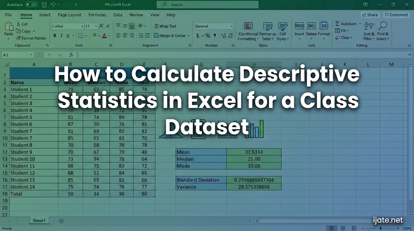
If you are working with a class dataset and need to summarize it numerically, Excel can handle the heavy lifting. Knowing how to calculate descriptive statistics in Excel for a class dataset saves you from crunching numbers by hand and gives your instructor a clean, professional output table every time. Whether your data comes from a psychology survey, a biology lab experiment, or a business statistics assignment, the process is the same. This guide walks you through everything you need, from enabling the right add-in to interpreting every value in the output table so you can write up your results with confidence.
Table of Contents
Quick Answer: Calculating Descriptive Statistics in 6 Steps
Here is the fastest path to getting your summary statistics table in Excel:
- Enable the Data Analysis ToolPak add-in through File > Options > Add-ins.
- Organize your class data in a single column with a header label in the first cell.
- Go to the Data tab on the Excel ribbon and click Data Analysis.
- Select Descriptive Statistics from the list and click OK.
- Set your Input Range to the data column, check Labels in first row, and tick Summary statistics.
- Choose an Output Range cell and click OK to generate the table.
These steps work in Excel 2016, 2019, 2021, and the desktop version of Excel 365. The entire process takes less than two minutes once the Data Analysis ToolPak is enabled. If you need more detail on any step, the sections below cover each one in depth.
What Are Descriptive Statistics?
Descriptive statistics are numerical measures that summarize the main features of a dataset. They give you a snapshot of your data so you can describe its shape, center, and spread without listing every individual value. Instead of reporting 50 separate test scores, you can report the average, the spread, and the range in a single paragraph.
There are two broad categories. Measures of central tendency tell you where the data clusters around a typical value. Measures of dispersion tell you how spread out the data points are from that center. Together, these two groups of statistics provide a complete picture of your class dataset.
For a class dataset, descriptive statistics are especially useful. Whether you are analyzing survey responses, test scores, reaction times, or experimental measurements, these summary values help you write a clear results section for your lab report or assignment. They also help your instructor verify that you worked with the full dataset rather than just eyeballing a few numbers. Most academic assignments in statistics, psychology, biology, and business courses expect you to report at least the mean, median, and standard deviation of your data.
Measures of Central Tendency: Mean, Median, and Mode
The three primary measures of central tendency are the mean, the median, and the mode. Each captures a slightly different picture of your data, and choosing the right one depends on the nature of your class dataset.
The mean is the arithmetic average. Excel calculates it with the =AVERAGE() function. Add up every value and divide by the number of values. The mean is sensitive to outliers, so a single extreme score can pull it away from the center of the rest of your data. For example, if most students scored between 70 and 85 but one scored 30, the mean will drop noticeably while the median stays near the cluster.
The median is the middle value when your data is sorted from lowest to highest. Excel uses =MEDIAN() for this. The median ignores outliers, so it is often a better measure of center when your class dataset has a few extreme values. Report the median when your data is skewed or when you want to describe the typical experience of the average student.
The mode is the most frequently occurring value in your dataset. Excel uses =MODE.SNGL() for a single mode or =MODE.MULT() if multiple values tie. The mode is most useful for categorical or discrete data, such as the most common test score, the most popular survey response option, or the most frequent classification in your data.
Measures of Dispersion: Range, Variance, and Standard Deviation
Central tendency tells you where your data sits. Dispersion tells you how tightly or loosely the values cluster around that center. Two datasets can have the same mean but very different spreads, so dispersion measures are essential for a complete description.
The range is the simplest measure. It is the difference between the maximum and minimum values in your dataset. A large range suggests your data spans a wide interval. The range is easy to calculate but is also sensitive to outliers, because it only uses the two most extreme values.
The variance measures the average squared distance of each data point from the mean. Excel offers =VAR.S() for sample variance and =VAR.P() for population variance. Because variance is in squared units, it is not always intuitive to report directly. For example, if your data is measured in points, the variance will be in points squared.
The standard deviation is the square root of the variance. Excel calculates it with =STDEV.S() for sample data and =STDEV.P() for population data. Standard deviation returns to the original units of your data, making it the most commonly reported dispersion measure in student assignments. A small standard deviation means most values are close to the mean. A large standard deviation means the data is widely scattered.
Excel also reports the standard error, which estimates how far the sample mean is likely to be from the true population mean. The skewness value tells you whether your data is symmetrical, stretched toward higher values, or stretched toward lower values. Kurtosis describes how peaked or flat your data distribution is compared to a normal curve. These two measures are more advanced but can add depth to your analysis if your assignment requires it.
How to Enable the Data Analysis ToolPak
The Data Analysis ToolPak is the quickest way to generate a complete descriptive statistics table in Excel. It is not always turned on by default, so you may need to enable it first. The entire process takes about thirty seconds.
Open Excel and click File in the top-left corner. Select Options from the bottom of the menu. In the Excel Options window, click Add-ins on the left sidebar.
Look at the Manage drop-down at the bottom of the window. If it says Excel Add-ins, click Go next to it. If it says something else, change it to Excel Add-ins first, then click Go.
In the Add-ins dialog box, check the box next to Analysis ToolPak. Click OK. Excel may take a moment to install the add-in.
Once installed, you should see a Data Analysis button in the Analysis group on the Data tab of the ribbon. If you still do not see it, close and reopen Excel completely. On a Mac, the steps are slightly different. Go to Tools, then Excel Add-ins, check Analysis ToolPak, and click OK. Note that Excel for Mac and Excel Online may not support the full Data Analysis ToolPak. If you are using a lab computer or a shared system, the ToolPak may already be enabled by your administrator.
Step-by-Step: Calculate Descriptive Statistics in Excel
With the Data Analysis ToolPak enabled, generating your descriptive statistics table takes just a few clicks. Follow these steps carefully to avoid common errors.
Step 1. Prepare your data. Enter your class dataset into a single column in Excel. Put a clear label in the first cell of that column, such as “Test Scores” or “Survey Responses.” Make sure every value in the column is numeric. Text entries, blank cells, or error values will cause the tool to fail or skip those rows.
Step 2. Open the Data Analysis dialog. Click the Data tab on the Excel ribbon. In the Analysis group, click Data Analysis. If you do not see Data Analysis, return to the enable steps above and make sure the ToolPak is properly installed.
Step 3. Select Descriptive Statistics. Scroll through the list of analysis tools and click Descriptive Statistics. Click OK to open the tool’s settings dialog box.
Step 4. Set the Input Range. Click the small selection button next to the Input Range field. Then click and drag to select your entire data column, including the header label. The range should appear in the format $A$1:$A$35 or similar, depending on your column and row numbers. If you accidentally select an extra empty row at the bottom, the ToolPak may include it as a zero value in your calculations.
Step 5. Choose output options. Check the box labeled Labels in first row if your selection includes the column header. This ensures the output table uses your label instead of a generic name. Check Summary statistics to generate the full set of measures including mean, median, mode, standard deviation, variance, and more. You can also check Confidence Level for Mean if your assignment requires a 95 percent confidence interval.
Step 6. Select the Output Range. Click the radio button next to Output Range. Click the selection button and click an empty cell where you want the results table to appear. Leave at least fifteen rows of empty space below that cell, because the output table is fairly tall and needs room to display all rows.
Step 7. Generate the output. Click OK. Excel will create a formatted table with your descriptive statistics in the location you chose. The table includes the statistic name in the first column and the computed value in the second column.
How to Interpret the Descriptive Statistics Output
The output table from the Data Analysis ToolPak has two columns. The first column lists each statistic by name. The second column shows the computed value for your dataset. Here is what each row means for your class assignment.
The Mean row shows the average of all your data points. Report this as the central value of your dataset. The Median row shows the middle value. If the mean and median are far apart, your data may be skewed by outliers, and you should mention this in your write-up.
The Mode row shows the most frequently occurring value. If no value repeats, Excel may display #N/A, which simply means there is no mode.
The Standard Deviation and Variance rows describe the spread of your data. A smaller standard deviation means most values cluster close to the mean. A larger standard deviation means your data points are more scattered. Report the standard deviation in your results, as it is more interpretable than variance.
The Minimum and Maximum rows show the lowest and highest values in your dataset. The Range row is the difference between these two values. These are useful for describing the full span of your data.
The Sum row adds all values together. The Count row shows the number of data points you included. Always verify that the Count matches the number of observations you collected. The Standard Error row estimates the precision of your sample mean.
The Sample Variance and Sample Standard Deviation rows use the sample formulas, dividing by n minus 1. These are the correct values to report for most class datasets where you are working with a sample rather than an entire population. The population versions divide by n instead and are only appropriate when your dataset includes every member of the group you are studying.
For your assignment, you typically need to report the mean, median, standard deviation, and range. Add skewness and kurtosis if your instructor specifically asks for them. Always state whether you used sample or population formulas, and confirm that your n matches the number of data points you collected. A well-written results paragraph might read: “The class dataset contained 35 observations with a mean of 78.4, a median of 79.0, and a standard deviation of 12.6, indicating moderate spread around the center.”
Using Individual Excel Functions as an Alternative
If the Data Analysis ToolPak is not available on your computer, you can still calculate descriptive statistics using individual Excel functions. This approach takes longer for a full set of statistics but works on every version of Excel without any add-in.
=AVERAGE(range) returns the mean. =MEDIAN(range) returns the median. =MODE.SNGL(range) returns the most frequent value. =STDEV.S(range) returns the sample standard deviation. =VAR.S(range) returns the sample variance. =MIN(range) and =MAX(range) give you the extreme values.
Type each formula in its own cell next to your data column. You can label them manually to create your own summary table. This method also works well if you only need a subset of statistics for a specific assignment question. For example, if your assignment only asks for the mean and standard deviation, two formulas are faster than running the full Data Analysis tool.
Tips for Class Dataset Analysis
Always label your data column before running the analysis. A clear header prevents confusion when you review the output table later. Double-check that every cell in your input range contains a number. Hidden text entries, spaces, or blank cells will cause the ToolPak to skip rows or throw an error that can be hard to track down.
Save a copy of your original data before running the analysis. The Data Analysis ToolPak does not modify your source data, but it is good practice to keep an untouched version in case you need to re-run the statistics with corrections. Keep your raw data on one sheet and your output table on a separate sheet for clarity.
When writing up your results, include the sample size n along with the mean and standard deviation. A common format is: “The dataset contained 35 observations with a mean of 78.4 and a standard deviation of 12.6.” This gives your reader the full context in one sentence. Always round your reported values to a reasonable number of decimal places. Two decimal places is standard for most class assignments.
Troubleshooting Common Issues
If the Data Analysis button does not appear on the Data tab, the ToolPak may not be enabled. Return to File > Options > Add-ins and confirm that Analysis ToolPak is checked under the Excel Add-ins section. Restart Excel after enabling it. The button should appear in the Analysis group on the Data tab.
If you see the error “Compile error in hidden module: Analysis,” your ToolPak installation may be corrupted. Remove the add-in, close Excel completely, reopen it, and re-enable the ToolPak. This error is common on older Excel versions and on Mac installations. Make sure you download the latest updates from Microsoft if the problem persists.
If your input range is not being recognized, make sure you selected the entire column including the header. The range must be entered in absolute reference format, such as $A$1:$A$30. Avoid using merged cells or tables with summary rows inside your input range. Excel will not process data inside an Excel Table object correctly with the ToolPak.
If your output overlaps with existing data, choose a different Output Range cell. The descriptive statistics table needs about fifteen rows of empty space. If your output range falls on top of existing data, Excel will overwrite those cells without warning. Always verify that the destination area is completely empty before clicking OK.
For non-numeric data, remove or separate text entries before running the analysis. The ToolPak only processes numeric values. If your class dataset includes text responses or categorical labels mixed in with numbers, consider running statistics on the numeric questions separately and handling the text data through frequency counts or pivot tables instead.
Descriptive Statistics for Multiple Columns at Once
The Data Analysis ToolPak can process more than one column in a single run. This saves time when your class dataset includes multiple variables such as several survey questions, multiple measurement columns, or grouped experimental data.
Select all the columns you want to analyze as your Input Range, making sure the first row of each column contains a label. Check the Labels in first row box. The output table will group the statistics by column, with each variable appearing in its own block of rows. This makes it easy to compare the summary statistics across different variables side by side.
This approach is especially useful for larger class datasets where you have collected responses to ten or more survey questions. You get a full summary for every column without repeating the steps for each one. Simply verify that each column contains only numeric values before running the analysis.
Excel 365 and Excel Online Considerations
The desktop version of Excel 365 includes the Data Analysis ToolPak and works the same way as Excel 2019 and 2021. The steps to enable the add-in and run descriptive statistics are identical. If you have a Microsoft 365 subscription, you already have access to the ToolPak.
If you use Excel through a web browser via Office.com, the Data Analysis ToolPak is not available. You will need to use individual functions like =AVERAGE() and =STDEV.S() instead, or download the file and open it in the desktop app to run the full analysis. This is an important limitation for students who primarily work on Chromebooks or shared lab computers with only the online version.
Mac users can enable the ToolPak through Tools > Excel Add-ins. However, some features may behave slightly differently on macOS compared to Windows. The dialog boxes may look different, and certain add-ins have historically had compatibility issues on the Mac platform. If you encounter problems, the individual function approach is a reliable fallback that works identically on all platforms.
Frequently Asked Questions
How do I calculate Descriptive Statistics in Excel?
How do you do Descriptive Statistics in Excel for grouped data?
How to calculate Descriptive Statistics?
How can Microsoft Excel be utilized for generating Descriptive Statistics?
Conclusion
Calculating descriptive statistics in Excel for a class dataset is straightforward once the Data Analysis ToolPak is enabled. The key steps are organizing your data in a labeled column, selecting the correct input and output ranges, and checking the Summary statistics option. Once the table appears, each row corresponds to a specific measure such as mean, median, standard deviation, or variance. Interpreting those values correctly is what turns raw numbers into meaningful results for your assignment. If you run into issues with the ToolPak, individual Excel functions provide a reliable backup that works on any version of Excel.