
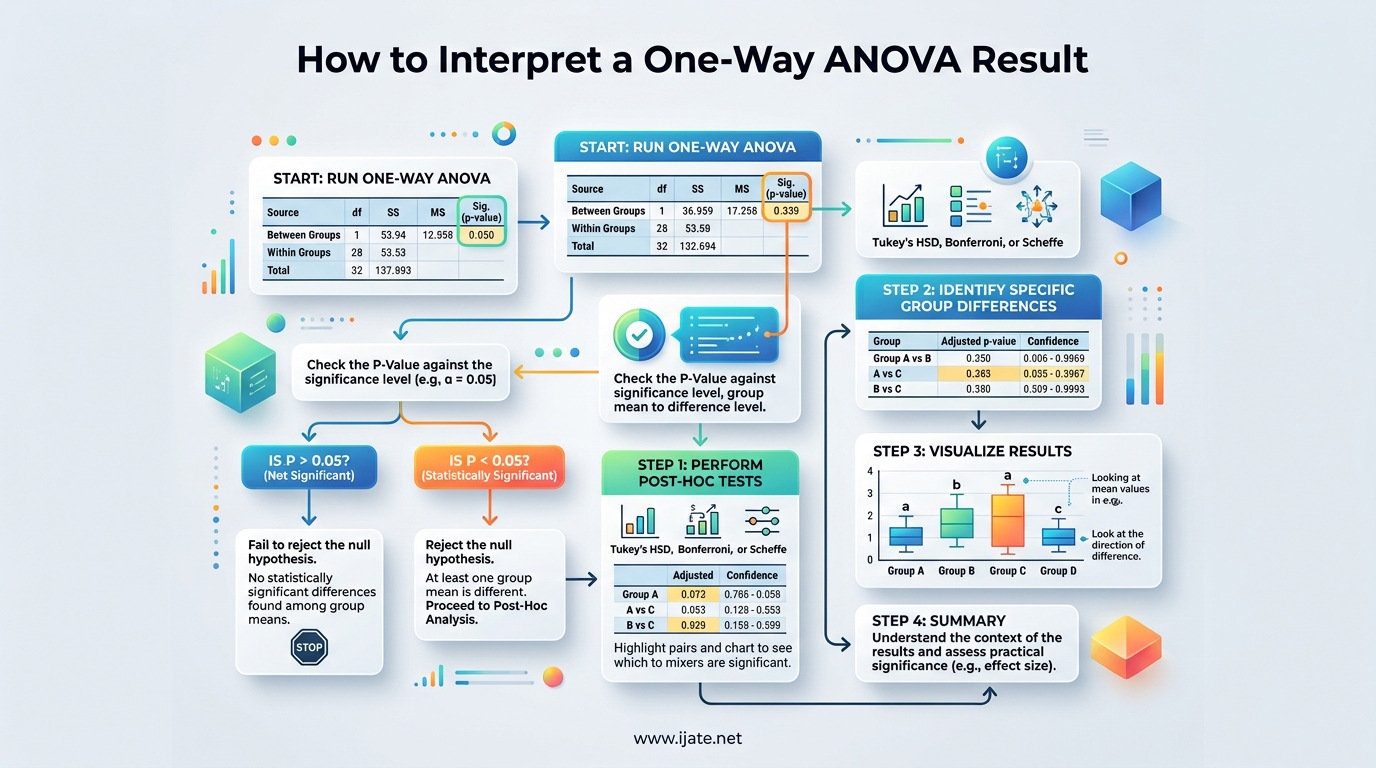
Learning how to interpret a one-way ANOVA result can feel overwhelming the first time you stare at an output table full of abbreviations like SS, MS, df, F, and p. I remember running my first ANOVA in a graduate statistics course and having no idea which numbers actually mattered. The good news is that once you understand the three-step framework, the process becomes almost automatic.
A one-way ANOVA (analysis of variance) tests whether the means of three or more independent groups differ significantly from each other. It is one of the most common statistical tests used in psychology, education, business, biology, and social science research. If you are comparing test scores across three teaching methods, for example, a one-way ANOVA tells you whether at least one group mean differs from the others.
In this guide, I will walk you through how to interpret a one-way ANOVA result step by step. We will cover the ANOVA table line by line, the p-value and F-statistic, post-hoc tests, effect size, assumption checks, and how to write up your findings in APA style. By the end, you will be able to read any ANOVA output with confidence.
Table of Contents
Quick Reference: The 3-Step ANOVA Interpretation Framework
Before we dive deep, here is the quick version. Every one-way ANOVA interpretation follows the same three steps:
Step 1 – Check for statistical significance: Look at the p-value in the ANOVA table. If it is less than your alpha level (usually 0.05), the differences between group means are statistically significant.
Step 2 – Examine the group means: Look at the descriptive statistics to see which groups have higher or lower averages and how wide the confidence intervals are.
Step 3 – Run post-hoc tests: If the overall ANOVA is significant, use a post-hoc test like Tukey HSD to find out exactly which pairs of groups differ from each other.
Those three steps answer the core questions: Is there a difference? Where does the difference appear? And which specific groups are different? Now let us go through each one in detail.
What a One-Way ANOVA Actually Tells You
A one-way ANOVA tests one fundamental question: do the means of three or more independent groups come from the same population, or do at least one pair come from different populations? The “one-way” part means there is a single categorical independent variable (the factor) with three or more levels (the groups).
The test works by comparing two types of variance. Between-group variance measures how far each group mean sits from the overall grand mean. Within-group variance measures how much individual scores deviate from their own group mean. The F-statistic is simply the ratio of these two variances.
If the between-group variance is much larger than the within-group variance, F will be large, suggesting that the groups genuinely differ. If the two variances are similar, F will be close to 1, suggesting no real difference between groups.
The null hypothesis in a one-way ANOVA states that all group means are equal. The alternative hypothesis states that at least one group mean differs from the rest. Notice that ANOVA does not tell you which specific groups differ, only that a difference exists somewhere.
That is why post-hoc tests exist. They come into play only after the overall ANOVA confirms a significant difference, helping you pinpoint exactly where the differences lie. See how ANOVA was applied in this published study for a real-world example of the test in action.
Step 1: Determine Whether Differences Are Statistically Significant
The first thing I do when interpreting ANOVA output is locate the p-value. This single number answers the most important question: is there a statistically significant difference between my groups?
Reading the ANOVA Table
Every software package – whether SPSS, R, Jamovi, Minitab, or GraphPad – produces an ANOVA table with the same core columns. Here is what each one means:
Source: This column lists where the variance comes from. You will see “Between Groups” (or “Treatment”) and “Within Groups” (or “Error”). Some tables also include a “Total” row.
DF (Degrees of Freedom): The between-groups degrees of freedom equals the number of groups minus one (k – 1). The within-groups degrees of freedom equals total sample size minus number of groups (N – k). These numbers determine the shape of the F-distribution used to calculate the p-value.
SS (Sum of Squares): This represents the total variability attributed to each source. SS Between captures variability due to group membership. SS Within captures variability due to individual differences and random error.
MS (Mean Square): Each MS is the sum of squares divided by its degrees of freedom. MS Between reflects the average variance between groups, and MS Within reflects the average variance within groups.
F (F-statistic): This is MS Between divided by MS Within. A larger F value means the between-group differences are large relative to the within-group variability. As a rough rule, F values above 4 with moderate sample sizes often indicate significance, but always rely on the p-value rather than eyeballing F.
P-value (Sig.): This is the probability of observing an F-statistic at least this large if the null hypothesis were true. A small p-value means the observed group differences are unlikely to be due to chance alone.
Interpreting the P-Value Against Your Alpha Level
The alpha level is your threshold for deciding whether a result is statistically significant. The conventional alpha level in most fields is 0.05, which means you accept a 5% risk of concluding that a difference exists when there is no actual difference (this is called a Type I error).
Here is the decision rule: if the p-value is less than or equal to your alpha level, you reject the null hypothesis and conclude that not all group means are equal. If the p-value is greater than alpha, you fail to reject the null hypothesis, meaning you do not have enough evidence to say the groups differ.
For example, if your ANOVA output shows F(2, 87) = 5.43, p = .006, the p-value of .006 is well below .05. You would reject the null hypothesis and conclude that at least one group mean differs significantly from the others.
One important caution: a significant p-value only tells you that a difference exists somewhere among your groups. It does not identify which groups differ. That is what post-hoc tests are for, which we will cover in Step 3.
What If the P-Value Is Not Significant?
If your p-value is above 0.05, you fail to reject the null hypothesis. This does not prove the groups are identical. It means your data did not provide strong enough evidence to conclude a difference exists. The groups might truly be similar, or your sample size might be too small to detect a real difference (low statistical power).
When results are non-significant, check your sample size. Small samples make it hard to detect even meaningful differences. Also examine the group means – if they look different but the p-value is not significant, a power issue may be at play.
Step 2: Examine the Group Means
Once you know a significant difference exists, the next step is looking at the actual group means to understand the direction and magnitude of the differences. The ANOVA table does not show you the means themselves – you need the descriptives or summary statistics table.
The Descriptives Table
Most software produces a descriptives table that shows, for each group: the mean, standard deviation, standard error, and a 95% confidence interval for the mean. This table is where you start understanding your results in a meaningful way.
Look at which groups have the highest and lowest means. For instance, if you are comparing three teaching methods and Method C has a mean exam score of 82 while Methods A and B sit at 68 and 71, Method C is clearly the standout. The descriptive statistics give you the real-world context that the F-statistic and p-value cannot provide alone.
Using Confidence Intervals
Confidence intervals around each group mean tell you about the precision of your estimates. Wide intervals suggest high variability within the group, while narrow intervals suggest more precise estimates. If the confidence intervals of two groups do not overlap, those groups are likely significantly different from each other.
Be careful with overlapping intervals, though. Overlapping confidence intervals do not automatically mean the groups are not significantly different. The formal test for that comes from the post-hoc comparisons, which we will discuss next.
Visualizing Group Means
I always recommend plotting your group means. A simple bar chart with error bars, or a box plot for each group, makes interpretation far easier than staring at numbers in a table. Many software packages generate these plots automatically as part of the ANOVA output.
Look for patterns: do the groups cluster together, or does one stand apart? Are there visible outliers? Visual inspection often reveals patterns that the summary statistics obscure.
Step 3: Compare Specific Groups With Post-Hoc Tests
A significant overall ANOVA tells you that at least one group differs, but it cannot tell you which ones. That is the job of post-hoc tests. These are follow-up pairwise comparisons that control the family-wise error rate, preventing the inflated Type I error that would occur if you ran separate t-tests on every pair.
Tukey HSD
Tukey’s Honestly Significant Difference (HSD) test is the most popular post-hoc test for one-way ANOVA. It compares every possible pair of group means while controlling the overall error rate at your alpha level. In SPSS and Jamovi, the output shows adjusted p-values for each pair.
To interpret Tukey results, look at the adjusted p-value for each pair. If the adjusted p-value is below 0.05, that specific pair of groups differs significantly. The output also shows the mean difference between each pair and a 95% confidence interval for that difference.
Some software packages also provide grouping letters. Groups that share a letter are not significantly different from each other. Groups with different letters are significantly different. For example, if Group A gets letter “a”, Group B gets letter “ab”, and Group C gets letter “b”, then Groups A and C differ significantly, while A and B, and B and C, do not.
Bonferroni Correction
The Bonferroni correction is a more conservative alternative. It divides your alpha level by the number of comparisons being made. If you have four groups, that means six pairwise comparisons, and the Bonferroni-adjusted alpha would be 0.05 divided by 6, or approximately 0.008.
Bonferroni is useful when you want to be extra cautious about false positives, but it reduces statistical power. This means you might miss real differences, especially with smaller samples. I recommend Tukey HSD as the default for most situations and Bonferroni when you have specific reason to minimize Type I error.
Other Post-Hoc Tests
Several other post-hoc tests exist for specific situations. Scheffe’s test is very conservative and works for complex comparisons beyond simple pairs. Dunnett’s test compares each group against a single control group rather than all pairs. Games-Howell is appropriate when the assumption of equal variances is violated.
For most one-way ANOVA situations with three to five groups and roughly equal sample sizes, Tukey HSD is the standard choice. It balances power and error control well, and reviewers in most academic fields expect to see it.
Interpreting Non-Significant Post-Hoc Results
Occasionally, you will get a significant overall ANOVA but no significant post-hoc comparisons. This paradox happens when the overall test detects differences across all groups simultaneously, but no single pair is different enough to pass the stricter post-hoc threshold.
In this case, report the significant overall ANOVA result and note that post-hoc tests did not identify specific group differences. This suggests the groups differ collectively rather than in pairwise fashion.
Effect Size: Going Beyond the P-Value
A significant p-value tells you that a difference exists, but it does not tell you how large that difference is. This is where effect size comes in. Effect size measures the magnitude of the difference between groups, independent of sample size.
Eta-Squared
The most common effect size for one-way ANOVA is eta-squared (written as n squared). It represents the proportion of variance in the dependent variable that is explained by group membership. Eta-squared ranges from 0 to 1.
Standard benchmarks for eta-squared are: 0.01 is considered a small effect, 0.06 is medium, and 0.14 or above is large. If your eta-squared is 0.15, for example, group membership accounts for 15% of the variance in your outcome variable, which qualifies as a large effect.
Partial Eta-Squared
Partial eta-squared is similar but is more commonly reported in designs with multiple factors. For a one-way ANOVA, eta-squared and partial eta-squared are mathematically identical because there is only one factor. Some software reports one, some the other, but they give you the same number in a one-way design.
Why Effect Size Matters
Statistical significance depends heavily on sample size. With 500 participants, even a tiny difference between groups can produce a significant p-value. Effect size tells you whether that difference is meaningful in the real world.
Always report effect size alongside your p-value. Reviewers and readers want to know both whether a difference exists and how large it is. A statistically significant result with a tiny effect size may not be practically important.
For more on how effect size and statistical significance interact in published education research, see this ANOVA application in a real study on the Ijate site.
Checking the ANOVA Assumptions
Before you fully trust your ANOVA results, you need to verify that the test’s assumptions are met. ANOVA is fairly robust to minor violations, but serious violations can produce misleading results.
Assumption 1: Normality
The dependent variable should be approximately normally distributed within each group. You can check this with a histogram, a Q-Q plot, or formal tests like Shapiro-Wilk. Minor deviations from normality are usually acceptable, especially with larger sample sizes (30+ per group), thanks to the central limit theorem.
Severe skewness or extreme outliers in any group can distort your results. If normality is badly violated, consider a non-parametric alternative like the Kruskal-Wallis test.
Assumption 2: Homogeneity of Variance
The variance of the dependent variable should be roughly equal across all groups. This is called homoscedasticity. Levene’s test is the standard check: if Levene’s test is non-significant (p > 0.05), the variances are sufficiently equal.
If Levene’s test is significant, your variances are unequal. You can then use Welch’s ANOVA, which does not assume equal variances, or report the Brown-Forsythe correction. Both are available in most statistical software.
Assumption 3: Independence of Observations
Each observation must be independent of every other observation. This means no participant appears in more than one group, and the data from one participant does not influence another. This assumption cannot be tested statistically – it depends on your study design.
Random assignment in experimental designs typically satisfies independence. If you have repeated measures or paired data, you need a repeated-measures ANOVA instead of a one-way ANOVA.
Common Mistakes When Interpreting ANOVA Results
Over years of teaching and consulting on statistics, I have seen the same interpretation mistakes repeatedly. Here are the most common ones to avoid.
Mistake 1: Interpreting a Significant ANOVA as Proof That All Groups Differ
A significant F-statistic only tells you that at least one group differs from at least one other. It does not mean every group is different from every other group. You must run post-hoc tests to identify which specific pairs differ.
Mistake 2: Running Separate T-Tests Instead of ANOVA
If you have four groups and run six separate t-tests, your Type I error rate inflates well beyond 0.05. ANOVA with post-hoc tests exists specifically to control this error rate. Always use ANOVA when comparing three or more groups.
Mistake 3: Ignoring Effect Size
Reporting only the p-value is like describing a movie as “good” without saying how good. A p-value of .001 might come from a large effect or simply a large sample. Without effect size, readers cannot judge the practical importance of your findings.
Mistake 4: Using ANOVA for Only Two Groups
If you have only two groups, a t-test is the appropriate tool. ANOVA will give you the same result mathematically (F equals t squared in a two-group comparison), but t-test output is more straightforward and widely expected for two-group comparisons.
Mistake 5: Skipping the Assumption Checks
Many students report ANOVA results without ever checking normality or homogeneity of variance. If Levene’s test fails and you proceed with a standard ANOVA, your results may be unreliable. Always report your assumption checks alongside the main results.
How to Write Up Your ANOVA Results (APA Style)
Once you have interpreted your results, you need to report them clearly. APA style provides a standard format. Here is a fill-in-the-blank template:
“A one-way ANOVA was conducted to determine whether [dependent variable] differed across [number] levels of [independent variable]. The overall model was significant, F([df between], [df within]) = [F value], p = [p value], n squared = [effect size]. Tukey post-hoc comparisons indicated that [Group A] (M = [mean], SD = [sd]) scored significantly higher than [Group B] (M = [mean], SD = [sd]), p = [adjusted p]. No significant differences were found between [other pairs].”
Always report the F-statistic with both degrees of freedom in parentheses, the exact p-value (unless it is less than .001), and an effect size measure. If your result was not significant, simply state: “The overall model was not significant, F(df1, df2) = X, p = .XX, suggesting no significant differences between groups.”
Frequently Asked Questions
What does a one-way ANOVA tell us?
A one-way ANOVA tells you whether the means of three or more independent groups are statistically different from each other. It tests the null hypothesis that all group means are equal against the alternative that at least one group mean differs. It does not identify which specific groups differ; that requires post-hoc tests.
What is the significance level of 0.05 in ANOVA?
A significance level of 0.05 means you accept a 5% risk of concluding that a difference exists when there is no actual difference. If your p-value is less than or equal to 0.05, you reject the null hypothesis and conclude that not all group means are equal.
How do I know if my ANOVA results are significant?
Check the p-value in your ANOVA table. If the p-value is less than or equal to your alpha level (typically 0.05), the result is statistically significant. You can also compare the F-statistic to the critical F-value, but the p-value approach is more straightforward and widely used.
How do I report one-way ANOVA results?
Report the F-statistic with both degrees of freedom, the p-value, and an effect size. In APA format: F(df_between, df_within) = F-value, p = value, eta-squared = value. Follow with post-hoc test results identifying which specific groups differ, including adjusted p-values and mean differences.
What does the F-statistic mean in ANOVA?
The F-statistic is the ratio of between-group variance to within-group variance. A larger F value means the differences between group means are large relative to the variability within groups. An F value near 1 suggests the group means are similar.
When should I use post-hoc tests after ANOVA?
Run post-hoc tests only when your overall ANOVA is statistically significant. They identify which specific pairs of groups differ from each other while controlling the family-wise error rate. Tukey HSD is the most common choice for pairwise comparisons.
Conclusion
Knowing how to interpret a one-way ANOVA result comes down to a simple three-step process. First, check the p-value to determine statistical significance. Second, examine the group means to understand the direction and magnitude of differences. Third, use post-hoc tests to identify which specific groups differ from each other.
Remember to report effect size, check your assumptions, and avoid common mistakes like treating a significant ANOVA as proof that all groups differ. With this framework, you can confidently interpret ANOVA output from any software and write up your results in a way that is both statistically sound and practically meaningful.