How to Interpret a Shapiro-Wilk Normality Test? (September 2026) Complete Guide

Imagine you are running an A/B test on two landing page designs, and your conversion data looks slightly skewed. You fire up your statistical software, run a t-test, and then freeze. Did you check normality first? If the answer is no, your results might be built on a shaky foundation.

If you have ever run a normality test and stared at the output wondering what to do next, you are in the right place. Learning how to interpret a Shapiro-Wilk normality test is one of the most useful skills for anyone working with statistics, whether you are writing a thesis, analyzing experimental data, or building machine learning models.

I remember the first time I encountered this test during my own research. I had reaction time data from 35 participants, and the histogram looked reasonable. The Shapiro-Wilk test returned p = 0.04, and I panicked. Was my entire analysis doomed? That confusion is what led me to dig deep into what the test actually measures and why it sometimes flags data that looks perfectly fine.

The Shapiro-Wilk test tells you whether your data follows a normal distribution. That single answer shapes which statistical methods you can safely use downstream, from t-tests to ANOVA to linear regression.

In this guide, I walk you through every step of interpreting the test results. I cover the null hypothesis, the W statistic, p-value rules, common pitfalls with large sample sizes, and practical examples in both Python and SPSS.

By the end, you will know exactly what to do when your software spits out a p-value and a W statistic. You will also understand why the test sometimes flags perfectly reasonable data as non-normal, and what to do about it.

What Is the Shapiro-Wilk Normality Test?

The Shapiro-Wilk test is a statistical procedure that checks whether a sample of data comes from a normally distributed population. Samuel Sanford Shapiro and Martin Wilk first published it in 1965, and it has since become one of the most widely recommended normality tests in statistics.

Unlike visual methods such as histograms or Q-Q plots, the Shapiro-Wilk test gives you a definitive number to work with. That makes it appealing when you need an objective decision rather than a judgment call.

Researchers, data scientists, and analysts reach for this test most often when sample sizes are small, typically under 50 observations. Multiple studies have shown it holds more statistical power than alternatives like the Kolmogorov-Smirnov test for detecting departures from normality in smaller samples.

The test compares the order statistics of your sample, meaning the sorted data values, against the values you would expect to see if the data truly came from a normal distribution. The closer the match, the more confident you can be that your data is normal.

One way to think about it: imagine lining up your data points from smallest to largest and comparing that lineup to the lineup you would expect from a perfect bell curve. If the two lineups match closely, your data is likely normal. If they diverge, the test flags it.

Why Normality Matters

Many of the most common statistical techniques assume normality. Parametric tests like the independent samples t-test, paired t-test, one-way ANOVA, and ordinary least squares regression all rely on this assumption to produce valid results.

If your data violates normality and you proceed with a parametric test anyway, your p-values and confidence intervals may be unreliable. You could end up drawing conclusions that do not hold up under scrutiny.

That said, normality matters to varying degrees depending on context. Some tests are more sensitive to violations than others, and the central limit theorem offers a safety net for larger samples.

How the Shapiro-Wilk Test Works

To interpret the test results confidently, you need a basic grasp of what happens under the hood. The test produces two key outputs: the W statistic and a p-value. Understanding the math behind these numbers helps you make better decisions, especially in edge cases.

The Null Hypothesis

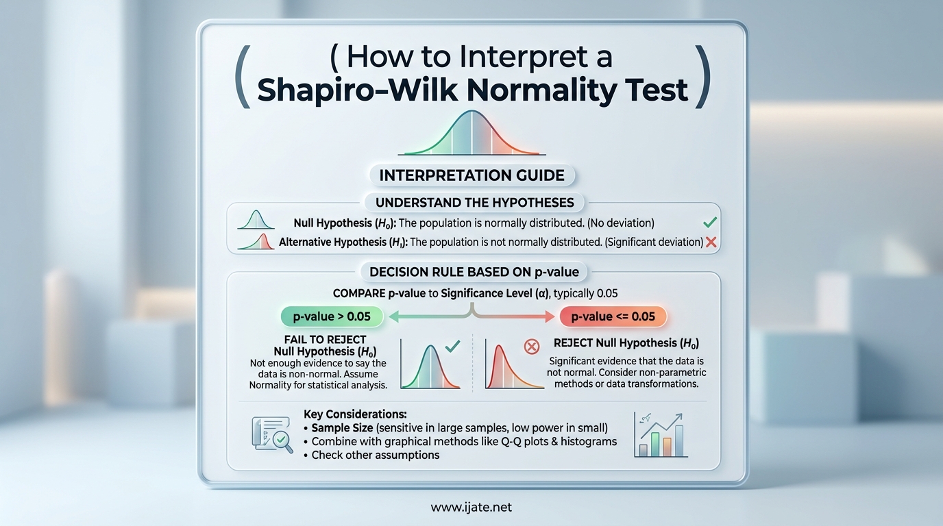
The Shapiro-Wilk test sets up a null hypothesis stating that your data is drawn from a normal distribution. The alternative hypothesis states that the data is not drawn from a normal distribution.

This framing is critical. The test can never prove that your data is normal. It can only fail to find evidence that it is not normal. That distinction trips up many researchers.

When the test returns a non-significant result, the correct interpretation is that you lack sufficient evidence to conclude your data deviates from normality. You do not get to claim you have proven normality.

Think of it like a criminal trial. The null hypothesis is “innocent until proven guilty.” A non-significant result means the prosecution did not present enough evidence to convict. It does not mean the defendant was proven innocent.

The W Statistic and Its Formula

The W statistic is the core output of the Shapiro-Wilk test. It ranges from 0 to 1, where a value of 1 indicates a perfect match to normality. Values closer to 0 indicate stronger departures from the normal distribution.

The formal definition of W is the ratio of the squared sum of a linear combination of order statistics to the sum of squared deviations from the sample mean. In simpler terms, the test sorts your data, multiplies each value by a specific weight derived from the expected normal order statistics, and compares that weighted sum to the total variance in your sample.

If we write this out, W equals the sum of squared differences between fitted and observed order statistics divided by the sum of squared deviations from the mean. The weights, often called coefficients, come from the inverse of the covariance matrix of normal order statistics. This is why the test is more computationally intensive than simpler alternatives.

The numerator captures how well a straight line fits your sorted data when plotted against expected normal values. The denominator captures total variability. When the fit is good, the ratio approaches 1. When the fit is poor, the ratio drops.

Most people do not need to calculate W by hand. Statistical software handles it automatically. What you need to know is that a higher W value means your data adheres more closely to a normal pattern.

One thing to watch for: the W statistic alone does not tell you whether the result is statistically significant. For that, you need the p-value.

Order Statistics Explained

Order statistics are simply your data points arranged from smallest to largest. If you have 10 observations, the first order statistic is your minimum value and the tenth is your maximum. The Shapiro-Wilk test uses these sorted values as the foundation of its calculation.

Under a normal distribution, each order statistic has an expected value and a known covariance structure with every other order statistic. The test leverages this known structure to assess whether your observed order statistics behave the way they should if the underlying population were normal.

This is fundamentally different from tests that look at skewness and kurtosis in isolation. The Shapiro-Wilk approach considers the entire shape of the distribution simultaneously, which is one reason it tends to be more powerful.

How the P-Value Is Derived

The p-value associated with the Shapiro-Wilk test represents the probability of observing a W statistic as extreme as the one you got, assuming the null hypothesis of normality is true.

A small p-value means the pattern in your data would be unlikely under normality. A large p-value means your data is consistent with what you would expect from a normal distribution.

The conversion from W to a p-value relies on approximation methods developed by Royston in 1982 and 1992. Royston’s work was a breakthrough because the original Shapiro-Wilk formulation only worked reliably for sample sizes up to 50. Royston introduced a transformation that converts W into an approximately standard normal variate, which makes p-value computation feasible for sample sizes up to several thousand.

Specifically, Royston showed that after a lognormal transformation of W, the resulting statistic follows a known distribution that can be approximated using polynomial fits calibrated against Monte Carlo simulations. This is what modern software implementations use behind the scenes.

For samples exceeding 5,000 observations, even Royston’s approximation starts to degrade. That is why scipy.stats.shapiro issues a warning at that threshold and why many statisticians recommend switching to visual methods or alternative approaches for very large datasets.

How to Interpret a Shapiro-Wilk Normality Test: Results

Here is where most people get stuck. The interpretation rules are actually straightforward once you memorize them, but the nuances can cause confusion. Let me break it down step by step.

The Quick Reference

If your p-value is greater than 0.05, you fail to reject the null hypothesis. This means your data is consistent with a normal distribution, and you can generally proceed with parametric tests.

If your p-value is less than or equal to 0.05, you reject the null hypothesis. This means your data shows a statistically significant departure from normality, and you should consider non-parametric alternatives or data transformations.

That two-line summary is the heart of how to interpret a Shapiro-Wilk normality test. Everything else is nuance and context.

Step 1: Locate the P-Value in Your Output

In SPSS, the Shapiro-Wilk result appears in the Tests of Normality table under the column labeled Sig. In Python using scipy.stats.shapiro, the p-value is the second element of the returned tuple. In R, the shapiro.test function prints the p-value directly.

Make sure you are reading the correct test column if your software reports multiple normality tests. SPSS commonly displays both Kolmogorov-Smirnov and Shapiro-Wilk results side by side.

Step 2: Check the W Statistic

While the p-value drives your decision, the W statistic gives you a sense of how far from normal your data is. A W of 0.98 with a significant p-value suggests a mild departure, while a W of 0.85 indicates a substantial deviation.

This context matters when you are deciding whether a transformation might fix the problem or whether you should switch to a non-parametric test entirely.

Step 3: Cross-Check With Visual Methods

I always recommend pairing the Shapiro-Wilk test with a Q-Q plot and a histogram. The test tells you whether a deviation exists, but the visuals show you what kind of deviation you are dealing with.

If the test flags non-normality but your Q-Q plot shows only minor wiggling at the tails, you may be dealing with a trivial departure that would not meaningfully affect your parametric analysis. This is especially common with larger sample sizes.

Step 4: Make Your Decision

Based on the p-value, the W statistic, and your visual inspection, you can now decide whether to proceed with parametric tests, transform your data, or switch to non-parametric alternatives like the Mann-Whitney U test or Kruskal-Wallis test.

Common Interpretation Mistakes

The biggest mistake I see is treating a non-significant result as proof of normality. Remember, failing to reject the null is not the same as accepting it. You simply do not have enough evidence to claim non-normality.

Another frequent error is ignoring sample size. With very large samples, the Shapiro-Wilk test becomes extremely sensitive and will flag even tiny, practically meaningless deviations from normality as statistically significant.

Conversely, with very small samples, the test lacks the power to detect even substantial departures from normality. You might get a non-significant result simply because you do not have enough data.

Practical Examples

Theory is useful, but nothing cements understanding like working through actual examples. Let me show you how to run and interpret the Shapiro-Wilk test in both Python and SPSS with real code you can copy and adapt.

Python Example Using scipy.stats.shapiro

Python is one of the most popular tools for running normality tests, and the scipy library makes it straightforward. Here is a complete walkthrough you can run yourself.

First, import the shapiro function from scipy.stats and create a sample dataset. You can generate normally distributed data using numpy to see what a clean result looks like:

import numpy as np
from scipy.stats import shapiro
data = np.random.normal(loc=100, scale=15, size=40)
stat, p = shapiro(data)

When you run this, you get two values back. The first is W, the test statistic, and the second is the p-value. For genuinely normal data with 40 observations, you will typically see W above 0.95 and p well above 0.05.

Now let us see what happens with clearly non-normal data. Generate a uniformly distributed sample instead:

data_skewed = np.random.uniform(low=0, high=100, size=40)
stat, p = shapiro(data_skewed)

Here you will likely see W drop below 0.95 and the p-value fall under 0.05, confirming a significant departure from normality. This side-by-side comparison is one of the fastest ways to build intuition for what the test detects.

To build a complete workflow, you can wrap the test in a simple decision function:

alpha = 0.05
if p > alpha:
    print(“Normal (fail to reject H0)”)
else:
    print(“Non-normal (reject H0)”)

One important note for Python users: recent versions of scipy.stats.shapiro display a warning when your sample size exceeds 5000. This is because the p-value approximation becomes unreliable at very large sample sizes. If your dataset is that large, consider visual methods or alternative approaches.

SPSS Example

In SPSS, you access the Shapiro-Wilk test through the Explore dialog. Go to Analyze, then Descriptive Statistics, then Explore. Move your variable into the Dependent List, click Plots, and check Normality plots with tests.

SPSS will produce a Tests of Normality table showing both Kolmogorov-Smirnov and Shapiro-Wilk results. Look at the Shapiro-Wilk row and find the Sig. column. That value is your p-value.

SPSS also generates a Q-Q plot alongside the test results, which gives you the visual cross-check I mentioned earlier. Use both pieces of information together for the most informed decision.

A common SPSS pitfall: if your sample size exceeds 2,000, SPSS may suppress the Shapiro-Wilk column and only show Kolmogorov-Smirnov results. This is a built-in limitation of older SPSS versions. In that case, switch to Python or R for your normality testing.

R Example

If you prefer R, the process is equally simple. The built-in shapiro.test function handles everything:

result <- shapiro.test(my_data)
print(result)

R prints both the W statistic and the p-value in a clean summary. You can also pipe the result into a visual check using ggplot2 to create a Q-Q plot with a reference line.

Reporting Results in APA Style

When writing up your results for a paper or thesis, APA style requires you to report the test statistic, degrees of freedom, and p-value. A typical Shapiro-Wilk write-up looks like this: the data were tested for normality using the Shapiro-Wilk test, and the results indicated no significant departure from normality, W = 0.97, p = .34.

If the test was significant, you would report that the data showed a significant departure from normality, W = 0.91, p = .003, and explain what you did next, such as applying a log transformation or using a non-parametric test.

Decision Tree: Choosing the Right Normality Approach

One thing I noticed across every competitor article I reviewed is that none of them provide a clear decision framework. They explain the test, but they leave you to figure out the decision logic on your own. Let me fix that gap.

Here is the decision tree I use when working through normality questions in my own analyses. It accounts for sample size, the type of test you plan to run, and the severity of any normality violation.

Step 1: Check Your Sample Size

If your sample size is under 50, the Shapiro-Wilk test is your best choice. It has the highest statistical power in this range, meaning it is most likely to detect genuine departures from normality without an excessive false positive rate.

If your sample size is between 50 and 500, Shapiro-Wilk is still appropriate, but you should weight the p-value alongside visual inspection more carefully. Start paying attention to the W statistic magnitude, not just significance.

If your sample size is between 500 and 5,000, the test remains mathematically valid but becomes increasingly sensitive. A significant p-value at this scale often reflects trivial deviations. Prioritize Q-Q plots and skewness or kurtosis values.

If your sample size exceeds 5,000, skip the formal test entirely. Rely on visual methods and the central limit theorem. The test will almost always return a significant result that tells you nothing useful.

Step 2: Run the Test and Check Visuals Together

Always run the Shapiro-Wilk test and a Q-Q plot at the same time. If they agree, your decision is straightforward. If they disagree, defer to the visual evidence when sample sizes are large.

Step 3: Decide Based on Your Downstream Test

If you are running a t-test or ANOVA with 30 or more observations per group, moderate non-normality is generally tolerable thanks to the central limit theorem. You can proceed with parametric tests even if the Shapiro-Wilk result is significant, as long as the deviation is not extreme.

If you are working with very small samples under 15 per group, take any significant Shapiro-Wilk result seriously. Switch to a non-parametric alternative or collect more data if feasible.

If you are checking regression residuals for normality, remember that only the residuals need to be normal, not the predictor or outcome variables themselves. This is a common point of confusion that leads to unnecessary alarm.

Limitations and Alternatives

The Shapiro-Wilk test is powerful, but it is not perfect. Understanding its limitations helps you use it more effectively and know when to look elsewhere.

The Large Sample Size Problem

This is the single biggest complaint I hear from researchers on forums like Reddit’s r/statistics. Users with sample sizes around 200 or more frequently report that the Shapiro-Wilk test flags their data as non-normal even when histograms and Q-Q plots look perfectly fine.

The reason is that as sample size increases, the statistical power of the test also increases. With enough data, the test can detect deviations from normality that are so small they have no practical consequence for your analysis.

This is why many statisticians recommend relying more heavily on visual inspection and effect size measures for large samples rather than treating the Shapiro-Wilk p-value as the final word.

The Central Limit Theorem Safety Net

Here is a concept that many guides gloss over. The central limit theorem states that as sample size grows, the sampling distribution of the mean approaches normality, regardless of the underlying population distribution.

This means that for many parametric tests, particularly those comparing means, normality of the raw data matters less as your sample size increases. With 30 or more observations per group, t-tests and ANOVA tend to be robust to moderate violations of normality.

This is why some statisticians argue that routine normality testing is of limited usefulness. For large samples, parametric tests are generally safe even when the Shapiro-Wilk test is significant, because the central limit theorem provides protection.

Shapiro-Wilk vs Kolmogorov-Smirnov

The Kolmogorov-Smirnov test is the most common alternative to Shapiro-Wilk, but it is generally less powerful for detecting departures from normality. Multiple simulation studies have confirmed that Shapiro-Wilk outperforms K-S, especially with smaller sample sizes.

The K-S test also requires you to specify the parameters of the normal distribution you are testing against, unless you use the Lilliefors correction. The Shapiro-Wilk test does not have this requirement, making it easier to use correctly.

For most practical situations, if you are choosing between the two, Shapiro-Wilk is the better default. Use K-S when you need to test against a distribution other than normal, or when you are working with very large datasets where Shapiro-Wilk becomes overly sensitive.

D’Agostino-Pearson Test

The D’Agostino-Pearson test, sometimes called the D’Agostino K-squared test, takes a different approach. Instead of looking at order statistics directly, it combines measures of skewness and kurtosis into a single test statistic.

This makes it conceptually easier to understand. If your data has near-zero skewness and kurtosis close to 3 (the values expected for a normal distribution), the test will not reject normality. If either measure deviates substantially, the test flags it.

The advantage of D’Agostino-Pearson is that it is less sensitive to the tail behavior that can trip up other tests. The disadvantage is that it may miss subtle shape departures that are not captured by skewness and kurtosis alone. In practice, it serves as a good complement to Shapiro-Wilk rather than a replacement.

Anderson-Darling Test

The Anderson-Darling test is another popular alternative. It is a modification of the Kolmogorov-Smirnov test that gives more weight to the tails of the distribution. This makes it particularly useful when you are concerned about extreme values pulling your analysis away from normality assumptions.

One key difference from Shapiro-Wilk: the Anderson-Darling test can be applied to any distribution, not just the normal. You simply change the reference distribution parameters. This flexibility makes it popular in quality control and engineering applications.

Simulation studies generally rank Anderson-Darling between Shapiro-Wilk and Kolmogorov-Smirnov in terms of power for detecting normality violations. It is a solid middle-ground choice if you want something more tail-sensitive than Shapiro-Wilk but more established than D’Agostino-Pearson.

Other Alternatives

Beyond those three, the Jarque-Bera test checks normality based on skewness and kurtosis and is popular in econometrics and financial modeling. It is simple to compute but generally less powerful than Shapiro-Wilk for small samples.

Each test has its strengths, but for general-purpose normality testing with small to moderate samples, Shapiro-Wilk remains the most recommended choice.

What to Do When Normality Is Violated

If your data fails the Shapiro-Wilk test and visual inspection confirms meaningful non-normality, you have several options. Data transformations like log, square root, or Box-Cox can sometimes normalize the distribution.

If transformations do not work, switch to non-parametric tests. The Mann-Whitney U test replaces the independent t-test, the Wilcoxon signed-rank test replaces the paired t-test, and the Kruskal-Wallis test replaces one-way ANOVA.

Bootstrapping is another powerful approach. It resamples your data to build an empirical sampling distribution, sidestepping the normality assumption entirely.

FAQs

Conclusion

Knowing how to interpret a Shapiro-Wilk normality test comes down to understanding two numbers: the W statistic and the p-value. A p-value above 0.05 means your data is consistent with normality, while a p-value at or below 0.05 signals a statistically significant departure.

Always pair the test with visual inspection, especially Q-Q plots and histograms. Sample size plays a huge role in how much weight you should give the p-value, so keep the large-sample sensitivity issue in mind.

Remember that the test cannot prove normality, it can only fail to find evidence against it. That philosophical distinction matters more than most people realize when interpreting results.

Your next step is to run the test on your own data using whatever tool you prefer. Once you have your results, use the decision framework in this guide to choose the right path forward, whether that means proceeding with parametric tests, transforming your data, or switching to non-parametric alternatives.