
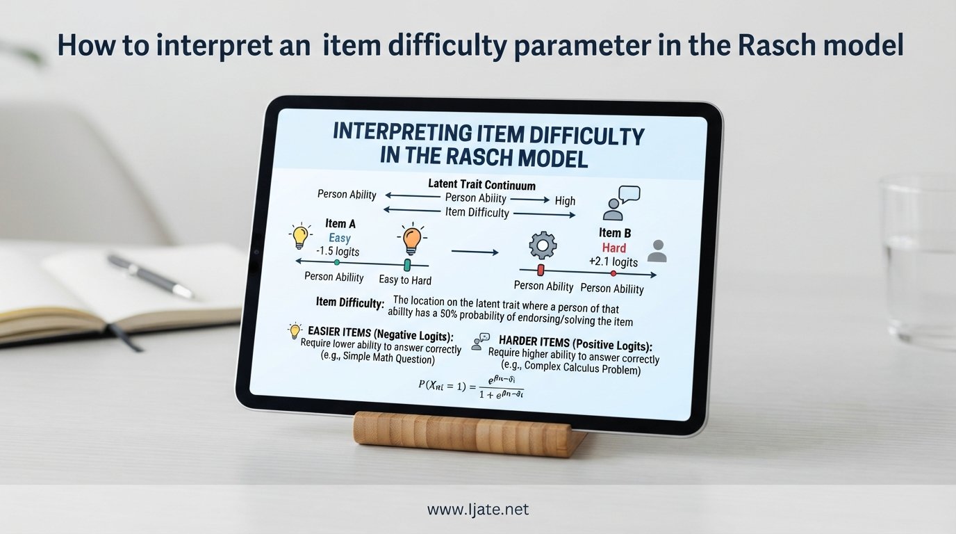
If you have ever stared at a Rasch model output and wondered what the numbers under “item difficulty” actually mean for your test, you are in the right place. The item difficulty parameter in the Rasch model tells you where each item sits on the ability scale, but reading those numbers correctly takes a bit of practice. Many researchers and graduate students confuse the sign of the value, mix it up with classical test theory statistics, or struggle to explain it to colleagues who have never studied item response theory. This guide walks through every step of interpretation so you can read your output with confidence and communicate results clearly to anyone.
By the end, you will understand what the difficulty parameter measures mathematically, how to translate specific values into plain language, and how to spot common mistakes before they reach a published report. If you work in educational assessment or psychometric analysis, this skill sits at the core of building fair, defensible tests. For related methodology on explanatory item response models, you can explore our published research collection.
Table of Contents
What Is the Item Difficulty Parameter in the Rasch Model?
The item difficulty parameter, usually written as b or sometimes β, marks the exact point on the latent ability scale where an examinee has a 50 percent probability of answering the item correctly. That definition sounds simple, but it carries a lot of information. The ability scale in a Rasch model typically runs from negative three to positive three, with zero representing the average ability level of the calibration sample. An item with b equal to zero is right in the middle: an average-ability person has a coin-flip chance of getting it right.
When b moves positive, the item becomes harder because a person needs more ability to reach that 50 percent threshold. When b moves negative, the item becomes easier because even lower-ability examinees can answer it correctly half the time. The parameter is sometimes called the “item location” because it literally locates the item on the same scale used to measure people. This shared scale is one of the defining features of Rasch measurement and is what allows direct comparison between items and between persons.
It is worth noting that the Rasch model treats difficulty as a property of the item itself, not of any particular group of examinees. This property is called “sample-free calibration” and it means the same item should show roughly the same b value whether you give it to high achievers or struggling students, provided the model fits. That stability is a major reason psychometricians choose Rasch over classical methods for high-stakes test construction.
The Mathematical Foundation
The Rasch model for dichotomous items uses a simple logistic equation to link person ability and item difficulty to the probability of a correct response. The formula reads: P(X = 1 | θ, b) = exp(θ − b) / (1 + exp(θ − b)). Here, θ (theta) is the person ability parameter and b is the item difficulty parameter. Both live on the same logit scale, which is why they can be subtracted directly.
When θ equals b, the exponent becomes zero, exp(0) equals one, and the formula returns one divided by two, or 0.50. That is the 50 percent probability point mentioned earlier. When θ is greater than b, the person has more ability than the item demands, so the probability climbs above 50 percent. When θ is less than b, the person has less ability than the item requires, and the probability drops below 50 percent.
The difference θ − b is the core of the model. It means the Rasch model only cares about the gap between person and item, not their absolute values. This is the property of “specific objectivity” that Georg Rasch emphasized. A two-logit gap produces the same probability whether the person is at +2 and the item at 0, or the person at 0 and the item at −2. The mathematics stays consistent across the entire scale.
One practical consequence is that the logit scale is symmetric and interval, not ordinal. A one-unit change in b represents the same shift in difficulty whether you are moving from −3 to −2 or from +1 to +2. This interval property is what justifies adding, subtracting, and averaging item difficulties in ways that would not be valid with raw percent-correct statistics.
How to Interpret Item Difficulty Parameter in the Rasch Model: Step-by-Step
Follow these five steps every time you read a new set of item difficulty estimates. The sequence works whether you are analyzing a 10-item quiz or a 200-item certification exam.
Step 1: Locate the item difficulty column in your output. In Winsteps this column is labeled “MEASURE” for items. In R packages like eRm or mirt it appears in the coefficient summary. Confirm the values are on the logit scale, not on a zero-to-one or zero-to-100 scale.
Step 2: Note the sign of each value. Positive values mean the item is harder than average. Negative values mean the item is easier than average. This is the single most common point of confusion because negative numbers often feel like “bad” results, but here a negative difficulty simply means an easy item.
Step 3: Translate the value into a probability statement. Subtract the item difficulty from a target ability level and plug the difference into the Rasch formula. For a quick estimate, remember that a difference of +1 logit gives roughly 73 percent probability, +2 logits gives about 88 percent, and −1 logit gives about 27 percent.
Step 4: Compare the item difficulty to your sample’s ability range. Items should spread across the ability distribution to measure precisely at every level. If all your items cluster near zero, you measure average examinees well but lose precision at the extremes. The test information function shows where your set of items is most and least informative.
Step 5: Flag items outside the typical range of −2 to +2 logits. Items beyond +2 are so hard that almost no one answers correctly, which wastes testing time. Items below −2 are so easy that almost everyone answers correctly, which adds no measurement information. Consider replacing or revising these items unless you need them for floor or ceiling coverage.
Following this checklist each time keeps interpretation consistent and catches errors before they propagate into test forms or research reports. Print it out, tape it next to your monitor, and work through it until the steps become automatic.
Positive vs Negative b-Values: What They Mean
A positive b-value means the item sits above the average ability level on the scale. Examinees need more ability than average to reach the 50 percent probability threshold. A value of +1.0, for example, means the item is appropriate for someone one logit above the mean. Using a rough z-score analogy, that corresponds to about the 84th percentile of the calibration sample.
A negative b-value means the item sits below the average ability level. The item is easy relative to the sample. A value of −1.0 means an examinee one logit below the mean has a 50 percent chance of answering correctly, roughly the 16th percentile. Beginners often assume negative means the item is flawed or scored incorrectly, but the sign only indicates direction on the ability scale.
Here is a quick reference for common values: b = 0 means the average examinee has a 50-50 chance. b = +0.5 is slightly harder than average. b = +1.5 is challenging, appropriate for above-average performers. b = −0.5 is slightly easier than average. b = −1.5 is very easy, appropriate for lower-ability examinees. Values beyond plus or minus two logits usually indicate items that contribute little measurement information for a typical sample.
Reading the Item Characteristic Curve (ICC)
The item characteristic curve is the visual representation of the Rasch probability formula. The horizontal axis shows ability, θ, usually running from −3 to +3 logits. The vertical axis shows the probability of a correct response, running from zero to one. The curve is always S-shaped, or sigmoidal, rising from near zero on the left to near one on the right.
The single most important point on the ICC is the inflection point, where the curve is steepest. In the Rasch model, this inflection point always sits exactly at probability 0.50, and the ability value at that point equals the item difficulty b. So when you look at an ICC, find where the curve crosses the 0.50 horizontal line, then read straight down to the ability axis. That number is the item difficulty.
Because the Rasch model fixes item discrimination at one, every ICC has the same slope at its inflection point. This means all Rasch ICCs are parallel, shifted only left or right by their difficulty values. When you overlay multiple Rasch ICCs on one graph, you see a family of identical S-curves marching across the ability scale. This visual parallelism is a quick diagnostic: if your curves have visibly different steepness, you may need a 2-PL model instead, or you may have items that violate Rasch assumptions.
Reading ICCs becomes intuitive with practice. A curve shifted far to the right represents a hard item. A curve shifted far to the left represents an easy item. The horizontal distance between any two curves tells you the difference in their difficulty values on the logit scale. For a deeper look at how Rasch analysis supports statistical adjustment of rater bias in Rasch analysis, our published research demonstrates these curves in applied settings.
Rasch Difficulty vs Classical Test Theory p-Value
Many newcomers to item response theory arrive with a background in classical test theory, where item difficulty is the p-value: the proportion of examinees who answered correctly. The p-value ranges from zero to one, and higher values mean easier items. This direction is opposite to the Rasch b-value, where higher values mean harder items.
The differences go deeper than direction. The p-value depends entirely on the sample that took the test. A difficult item given to strong students may show a high p-value, while the same item given to weaker students shows a low p-value. The Rasch b-value aims to be sample-independent, producing a stable difficulty estimate that holds across populations when the model fits.
Another difference is scale type. The p-value is a proportion, which is ordinal in nature; you cannot meaningfully add or subtract p-values. The Rasch logit scale is interval, so differences and averages are mathematically meaningful. This is why Rasch difficulty estimates support more sophisticated analyses, including test equating, item banking, and computerized adaptive testing.
Rasch Model vs 1-PL, 2-PL: Why Discrimination Matters
The Rasch model and the 1-parameter logistic model, or 1-PL, look almost identical mathematically. Both use only a difficulty parameter and fix discrimination at one. The distinction is philosophical. The Rasch model is a measurement model that requires this constraint to achieve specific objectivity. The 1-PL is a statistical model that happens to use the same formula but is chosen primarily for parsimony.
The 2-PL model adds a discrimination parameter, a, which lets each item have a different ICC slope. Items that discriminate well between high and low ability examinees get steeper curves. Items that discriminate poorly get flatter curves. This flexibility can improve model fit, but it sacrifices the specific objectivity that makes Rasch measurement distinctive.
From a practical standpoint, if your goal is to build a measurement scale where items and persons are comparable in a strict, additive sense, the Rasch model’s constraint is a feature, not a limitation. If your goal is purely statistical fit with a given dataset, a 2-PL may reduce misfit at the cost of generality. Researchers using differential item functioning (DIF) analysis with Rasch often prefer the constrained model because it isolates difficulty differences without confounding them with discrimination differences.
Practical Examples of Interpreting b-Values
Consider a 30-item mathematics test calibrated with the Rasch model. Suppose Item 5 has b = −1.2, Item 15 has b = 0.3, and Item 28 has b = +1.8. Each value tells a different story about who the item serves best.
Item 5, with b = −1.2, is an easy item. A student at −1.2 logits of ability has a 50 percent chance of answering correctly. A student at the mean, θ = 0, has a probability of about 77 percent. This item is well placed for distinguishing among lower-ability students. It provides useful information at the bottom of the ability range where harder items would be answered incorrectly by everyone and would add no measurement signal.
Item 15, with b = 0.3, is slightly harder than average. An average-ability student has a probability of about 43 percent. This item is well targeted at the middle of the distribution and is the type of item that does the heavy lifting in a typical test. Most of your measurement precision comes from items near the mean ability level.
Item 28, with b = +1.8, is a hard item. Even a student at +1 logit of ability has only about a 27 percent chance of answering correctly. Only students near +1.8 logits or higher reach the 50 percent mark. This item discriminates among top performers and is essential if your test needs to identify high achievers. Without items like this, your test would have a ceiling effect and could not distinguish between a good student and an exceptional one.
Common Mistakes and How to Avoid Them
Mistake 1: Treating negative b-values as errors. Negative values are normal and simply mean the item is easier than average. Do not delete or rescore these items without checking model fit statistics.
Mistake 2: Confusing Rasch difficulty with CTT p-value direction. Higher p-value means easier. Higher b-value means harder. Write this on a sticky note until it becomes second nature.
Mistake 3: Ignoring the calibration sample. Although Rasch aims for sample-free calibration, extreme samples can still produce unstable estimates. Always check the standard error of each item difficulty and the model fit statistics before interpreting.
Mistake 4: Reporting b-values without context. A bare number like b = 1.3 means little to a stakeholder. Translate it into a probability statement or a percentile equivalent so non-specialists can understand.
Mistake 5: Assuming all items must cluster near zero. A well-designed test spreads items across the ability range. Items at −1.5 and +1.5 are not outliers to be removed; they are necessary for measuring the full spectrum of ability.
FAQs
What does the item difficulty parameter mean in IRT?
The item difficulty parameter, written as b, marks the point on the latent ability scale where an examinee has a 50 percent probability of answering the item correctly. Higher b-values indicate harder items that require more ability.
How do you interpret item difficulty parameter b?
Read the sign and magnitude. A positive b means the item is harder than average and a negative b means it is easier than average. The absolute value tells you how far from the mean the item sits. Compare b to your sample ability range to confirm the item targets the right examinees.
What is the difference between the Rasch model and the 1-PL model?
Mathematically the two models use the same formula with discrimination fixed at one. The Rasch model is a measurement theory that requires this constraint to achieve specific objectivity, meaning item and person parameters can be compared additively. The 1-PL is a statistical model chosen for parsimony without the same measurement philosophy.
How do you interpret item characteristic curves?
Find where the curve crosses the 0.50 probability line and read down to the ability axis. That value is the item difficulty. In the Rasch model all curves share the same slope at this inflection point, so they are parallel shifts of each other across the ability scale.
Conclusion
Learning how to interpret an item difficulty parameter in the Rasch model opens the door to defensible, precise test construction. The parameter locates each item on the ability scale at the 50 percent probability point. Positive values signal harder items and negative values signal easier items, with the logit scale providing interval-level measurement that supports comparison, equating, and adaptive testing. By following the five-step interpretation checklist, reading ICCs for the inflection point, and avoiding the common mistakes outlined above, you can turn raw model output into clear, communicable insights.
Keep practicing with your own datasets. The more b-values you interpret in context, the faster the numbers translate into plain language. When you are ready to explore advanced applications, our research on explanatory item response models and DIF analysis extends these fundamentals into polytomous data and bias detection.