The Difference Between One-Way and Two-Way ANOVA in (2026)

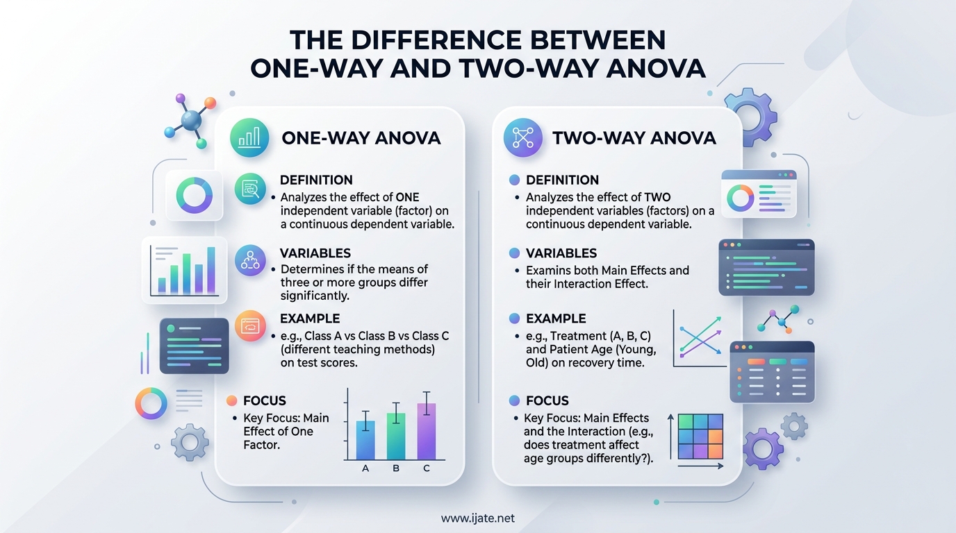
If you have ever stared at your research data and wondered which statistical test to use, you are in the right place. The difference between one-way and two-way ANOVA comes down to one simple thing: the number of independent variables you are testing. A one-way ANOVA evaluates how a single factor affects a continuous dependent variable, while a two-way ANOVA examines how two factors work separately and together to influence that same outcome.

That distinction sounds small, but it changes everything about your analysis. Pick the wrong one, and you could miss a critical interaction between variables or draw a conclusion that does not hold up under scrutiny. We have seen researchers run multiple one-way ANOVAs when a single two-way ANOVA would have been more powerful and more honest about what the data actually says.

The confusion is common enough that statistics forums like r/AskStatistics and stats.stackexchange.com are filled with threads asking why one-way and two-way ANOVA sometimes produce different results on the same dataset. The answer lies in how each test partitions variance, and we will explain that in plain language below.

In this guide, we break down both tests so you can make the right call for your own data. We cover definitions, assumptions, when to use each test, real examples, and common mistakes to avoid. For a published example of how ANOVA analysis is applied in academic research, the Ijate journal provides a useful reference.

What Is One-Way ANOVA?

One-way ANOVA (analysis of variance) is a statistical test that compares the means of three or more groups defined by a single categorical independent variable. You use it when you want to know whether different levels of one factor produce measurably different outcomes in a continuous dependent variable.

Think of it as a smarter version of the t-test. A t-test handles two groups, but when you have three or more, running multiple t-tests inflates your risk of a false positive. One-way ANOVA solves that problem by testing all groups simultaneously using a single F-statistic.

For example, imagine you want to compare the average test scores of students taught with three different methods: traditional lecture, flipped classroom, and project-based learning. Teaching method is your single independent variable with three levels. Student test score is your continuous dependent variable. One-way ANOVA tells you whether any of the three methods produce significantly different average scores.

The Core Logic of One-Way ANOVA

One-way ANOVA partitions the total variance in your data into two buckets. The first is between-group variation, which captures differences caused by your independent variable. The second is within-group variation, which captures natural differences among individual observations within each group.

The test then computes an F-ratio by dividing the mean square between groups by the mean square within groups. If that ratio is large enough, you reject the null hypothesis and conclude that at least one group mean differs from the others.

In statistical terms, the sum of squares between groups (SSB) measures how much the group means deviate from the grand mean. The sum of squares within groups (SSW) measures how much individual observations deviate from their respective group means. The F-ratio essentially asks whether the differences between groups are large relative to the natural spread within groups.

Hypotheses in One-Way ANOVA

Your null hypothesis states that all group means are equal. The alternative hypothesis states that at least one group mean is different from the others. Notice the wording carefully: rejecting the null does not tell you which specific groups differ, only that a difference exists somewhere among them.

That limitation is where post-hoc tests come in. Tukey’s HSD, Bonferroni correction, and Scheffe’s test help you pinpoint which specific pairs of groups differ after the overall ANOVA shows a significant result. Without a post-hoc test, your one-way ANOVA result is only half the story.

Choosing the right post-hoc test matters. Tukey’s HSD is a solid all-purpose choice when group sizes are equal. Bonferroni is more conservative and works well when you have a small number of comparisons. Scheffe’s test is the most flexible and handles unequal sample sizes, but it is also the least powerful.

Assumptions of One-Way ANOVA

You should confirm your data meets three core assumptions before running the test. Violating these assumptions can produce misleading results, so checking them is not optional.

• Normality: The dependent variable should be approximately normally distributed within each group. You can check this with a Shapiro-Wilk test or a Q-Q plot.
• Homogeneity of variance: Also called homoscedasticity, this means all groups should have roughly equal variances. Levene’s test is the standard tool for checking this assumption.
• Independence of observations: Each data point should be collected independently of the others. This is a design issue rather than something you can test after data collection, so it must be addressed during your experimental planning.

If these assumptions are seriously violated, consider a non-parametric alternative like the Kruskal-Wallis test. That test does not assume normality and is based on ranks rather than raw values.

What Is Two-Way ANOVA?

Two-way ANOVA does everything one-way ANOVA does, but it adds a second independent variable into the analysis. With two factors in play, the test evaluates three things simultaneously: the main effect of the first factor, the main effect of the second factor, and the interaction effect between them.

That third piece is what makes two-way ANOVA genuinely different from running two separate one-way tests. An interaction effect occurs when the impact of one variable depends on the level of the other. In other words, the two variables do not just add up independently. They combine in a way that changes the outcome in directions you might not expect.

Two-way ANOVA is sometimes called factorial ANOVA because it analyzes data from a factorial design where every level of one factor is crossed with every level of the other. This design creates a grid of group combinations that the test evaluates together in a single coherent model.

Understanding Interaction Effects

This is the concept that trips up the most students and researchers, so let us make it concrete with a healthcare example. Imagine you are testing two factors: medication type (Drug A versus Drug B) and patient age group (young versus old). A main effect would tell you that Drug A lowers blood pressure more than Drug B overall, averaged across all patients.

An interaction effect would tell you something far more nuanced and potentially more important. It might reveal that Drug A works much better for young patients but actually performs worse than Drug B for older patients. That crossover pattern is invisible to a one-way ANOVA because one-way tests have no mechanism to detect how two variables influence each other.

This is exactly why forum discussions on r/statistics and stats.stackexchange.com are filled with questions about why one-way and two-way ANOVA sometimes give different results on the same data. The two-way test partitions variance differently, accounting for the second factor and the interaction before evaluating each main effect individually.

If you run a one-way ANOVA on factor A alone, any variance actually caused by factor B gets lumped into the error term. That inflates your error variance and can mask a real effect. The two-way ANOVA pulls that variance out and attributes it correctly, giving you cleaner and more accurate results.

Hypotheses in Two-Way ANOVA

Two-way ANOVA tests three separate sets of hypotheses in a single analysis. First, it tests whether factor A has a significant main effect on the dependent variable, ignoring factor B. Second, it tests whether factor B has a significant main effect, ignoring factor A. Third, it tests whether the interaction between factor A and factor B is significant.

Each of these produces its own F-statistic and p-value. You might find a significant main effect for one factor, no effect for the other, and a significant interaction. All combinations are possible, and each tells a different story about your data.

When you do find a significant interaction, interpreting the main effects becomes more complicated. A significant interaction means the effect of one factor depends on the level of the other, so talking about the main effect of factor A in isolation can be misleading. In those cases, you should follow up with simple main effects analysis to understand the pattern.

Assumptions of Two-Way ANOVA

Two-way ANOVA requires the same three assumptions as one-way: normality, homogeneity of variance, and independence of observations. The dependent variable should be continuous and approximately normally distributed within each cell of your factorial design.

Additionally, the design should ideally be balanced, meaning each combination of factor levels has the same number of observations. Balanced designs make the math cleaner because the sums of squares for each factor and the interaction are orthogonal, meaning they do not overlap.

Unbalanced designs can still be analyzed, but they require careful decisions about which type of sums of squares to use. Type I, Type II, and Type III sums of squares handle unbalanced data differently, and the choice can affect your conclusions. Most statisticians recommend Type III sums of squares for unbalanced factorial designs because they test each effect after accounting for all other effects.

Key Differences: One-Way vs Two-Way ANOVA

Now let us put the two tests side by side. The table below summarizes the primary differences between one-way and two-way ANOVA so you can quickly identify which test fits your situation.

Feature	One-Way ANOVA	Two-Way ANOVA
Number of independent variables	1	2
Effects tested	Main effect only	Main effects for both factors plus interaction effect
Null hypotheses tested	1 (all group means are equal)	3 (factor A, factor B, and interaction)
F-statistics produced	1	3
Design type	Single-factor design	Factorial design
Can detect interaction effects?	No	Yes
Minimum groups compared	3	4 (2×2 factorial at minimum)
Complexity of interpretation	Lower	Higher
Variance partitioning	Between-group and within-group only	Factor A, Factor B, interaction, and error
Statistical power relative to sample size	Lower when two factors are involved	Higher because error variance is reduced

The most important row in that table is the interaction effect. This is the single biggest reason researchers choose two-way over one-way ANOVA. Without the ability to detect interactions, you could completely miss a pattern in your data where one variable changes the behavior of another.

Another critical difference involves statistical power. A two-way ANOVA uses all your data to estimate error variance, which typically gives you more power than running two separate one-way ANOVAs on the same factors. It also controls the familywise error rate better because you are running one unified test instead of multiple independent tests on the same dataset.

Finally, consider degrees of freedom. Two-way ANOVA consumes more degrees of freedom because it estimates effects for both factors and their interaction. With small sample sizes, this can reduce power. But with adequate sample sizes, the benefit of correctly partitioning variance far outweighs the cost of additional degrees of freedom.

Practical Examples of One-Way and Two-Way ANOVA

Examples make abstract concepts click. Here are two scenarios that illustrate when each test is the right choice and why choosing correctly matters.

One-Way ANOVA Example

Say you are a food scientist testing whether four different cookie recipes produce different sweetness scores on a 10-point scale. Recipe type is your single independent variable with four levels (Recipe A, B, C, and D). Sweetness score is your continuous dependent variable.

You collect ratings from 40 taste testers, with 10 testers assigned to each recipe. A one-way ANOVA compares the mean sweetness score across all four recipes simultaneously. If the F-statistic is significant at your chosen alpha level, you follow up with Tukey’s HSD to learn which specific recipes differ from each other.

Notice that there is no second factor here. You are not interested in how recipe type interacts with anything else. You just want to know which recipe produces the sweetest cookie. One-way ANOVA is exactly the right tool for this question.

Now suppose you tried to force a second factor into this analysis, like tester gender, just because you collected that information. Unless gender is genuinely relevant to your research question, adding it creates a more complex model without adding meaningful insight. The simpler one-way analysis is both cleaner and more appropriate.

Two-Way ANOVA Example

Now expand the cookie scenario. You still have four recipes, but you also want to know whether baking temperature (325 degrees versus 375 degrees) affects sweetness scores. Now you have two independent variables: recipe type with four levels and baking temperature with two levels.

A two-way ANOVA answers three questions in one analysis. Does recipe type affect sweetness scores overall, averaging across temperatures? Does baking temperature affect sweetness scores overall, averaging across recipes? And critically, does the effect of recipe type change depending on baking temperature?

That third question is where the real value of two-way ANOVA becomes apparent. You might discover that Recipe A is the sweetest at 325 degrees but actually the least sweet at 375 degrees. No amount of separate one-way ANOVAs could reveal that crossover pattern because the interaction between recipe and temperature only becomes visible when both factors are analyzed together in a single model.

This is why we always recommend two-way ANOVA over running multiple one-way tests when your experimental design includes two factors. The two-way approach is not just more convenient. It detects effects that separate one-way tests would entirely miss, and it does so with better statistical power.

When to Use One-Way vs Two-Way ANOVA

The decision comes down to your experimental design. If you are manipulating or observing one categorical variable, one-way ANOVA is sufficient. If you have two categorical variables and want to understand their individual and combined effects, two-way ANOVA is the correct choice.

One common mistake we see frequently on statistics forums is researchers running two separate one-way ANOVAs when they should run a single two-way ANOVA. This approach misses interaction effects entirely and reduces statistical power because each one-way test uses a smaller portion of the data to estimate error variance. The variance explained by the second factor gets absorbed into the error term, making real effects harder to detect.

Another mistake is jumping to two-way ANOVA when you only have one meaningful factor. Adding a second variable that is not relevant to your research question adds complexity without value, consumes degrees of freedom, and can make your results harder to interpret and communicate to your audience.

After any significant ANOVA result, always run a post-hoc test to identify which specific groups differ. For one-way ANOVA, Tukey’s HSD is a reliable default choice. For two-way ANOVA, you may need simple main effects analysis to unpack a significant interaction and understand exactly how one factor behaves at each level of the other.

Quick Decision Guide

Still unsure which test to use? Ask yourself these questions in order. How many categorical independent variables does my experimental design include? If the answer is one, use one-way ANOVA. If the answer is two, use two-way ANOVA.

Do I care whether the two variables interact? If yes, two-way ANOVA is the only option that can answer that question. If no and you genuinely have two separate research questions with no interest in their combined effect, running two one-way ANOVAs is defensible but still less efficient.

Is my design balanced? Two-way ANOVA works best with equal sample sizes in each cell. Unbalanced designs are manageable but require more careful analysis choices.

FAQs

Conclusion

The difference between one-way and two-way ANOVA is straightforward at its core. One-way handles a single factor, while two-way handles two factors along with their interaction effect. Choose based on your experimental design, not on which test seems simpler or faster to run.

When two factors are in play, two-way ANOVA gives you the full picture that separate one-way tests simply cannot deliver. It detects interactions, provides better statistical power, and partitions variance more accurately. Match the test to your design, check your assumptions, and always follow up with post-hoc analysis to get the most out of your data.